Chapter 11, Problem 32CE

Instructions: You may use Excel, MegaStat, Minitab, JMP, or another computer package of your choice. Attach appropriate copies of the output or capture the screens, tables, and relevant graphs and include them in a written report. Try to state your conclusions succinctly in language that would be clear to a decision maker who is a nonstatistician. Exercises marked * are based on optional material. Answer the following questions, or those your instructor assigns.

1. a. Choose an appropriate ANOVA model. State the hypotheses to be tested.
2. b. Display the data visually (e.g., dot plots or line plots by factor). What do the displays show?
3. c. Do the ANOVA calculations using the computer.
4. d. State the decision rule for α = .05 and make the decision. Interpret the p-value.
5. e. In your judgment, are the observed differences in treatment means (if any) large enough to be of practical importance?
6. f. Given the nature of the data, would more data collection be practical?
7. g. Perform Tukey multiple comparison tests and discuss the results.
8. h. Perform a test for homogeneity of variances. Explain fully.

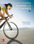
In a bumper test, three types of autos were deliberately crashed into a barrier at 5 mph, and the resulting damage (in dollars) was estimated. Five test vehicles of each type were crashed, with the results shown below. Research question: Are the mean crash damages the same for these three vehicles?