
a.
Find the value of the
a.
Answer to Problem 20E
The value of chi-square statistic is 0.965.
Explanation of Solution
Calculation:
The
Contingency table:
A contingency table is obtained as using two qualitative variables. One of the qualitative variable is row variable that has one category for each row of the table another is column variable has one category for each column of the table.
The hypotheses are:
Null Hypothesis:
Alternate Hypothesis:
Now, it is obtained that,
| Gender | Male | Female | Row Total |
| Optimistic | 1,148 | 815 | 1,963 |
| Pessimistic | 225 | 178 | 403 |
| Column Total | 1,373 | 993 | 2,366 |
Expected frequencies:
The expected frequencies in case of contingency table is obtained as,
Now, using the formula of expected frequency it is found that the expected frequency for the optimistic male is obtained as,
Hence, in similar way the expected frequencies are obtained as,
| Gender | Male | Female |
| Optimistic | ||
| Pessimistic |
Chi-Square statistic:
The chi-square statistic is obtained as
The accept and reject can be rewritten as,
| Male | 1 |
| Female | 2 |
Test Statistic:
Software procedure:
Step -by-step software procedure to obtain test statistic using MINITAB software is as follows:
- Select Stat > Table > Cross Tabulation and Chi-Square.
- Check the box of Raw data (categorical variables).
- Under For rows enter Row.
- Under For columns enter Gender.
- Check the box of Count under Display.
- Under Chi-Square, click the box of Chi-Square test.
- Select OK.
- Output using MINITAB software is given below:
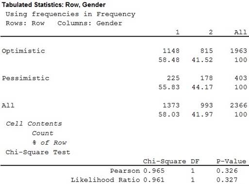
Thus, the value of chi-square statistic is 0.965.
b.
Find the proportion of men who were optimistic.
b.
Answer to Problem 20E
The proportion of men who were optimistic is 0.836.
Explanation of Solution
Calculation:
From part (a), it is found that,
| Gender | Male | Female | Row Total |
| Optimistic | 1,148 | 815 | 1,963 |
| Pessimistic | 225 | 178 | 403 |
| Column Total | 1,373 | 993 | 2,366 |
Hence, the proportion of men who were optimistic is,
Thus, the proportion of men who were optimistic is 0.836.
c.
Find the proportion of women who were optimistic.
c.
Answer to Problem 20E
The proportion of women who were optimistic is 0.821.
Explanation of Solution
Calculation:
From part (a), it is found that,
| Gender | Male | Female | Row Total |
| Optimistic | 1,148 | 815 | 1,963 |
| Pessimistic | 225 | 178 | 403 |
| Column Total | 1,373 | 993 | 2,366 |
Hence, the proportion of women who were optimistic is,
Thus, the proportion of women who were optimistic is 0.821.
d.
Find the test statistic z for testing the null hypothesis that the two proportions are equal versus the alternative that they are not equal.
d.
Answer to Problem 20E
The test statistic z for testing the null hypothesis that the two proportions are equal versus the alternative that they are not equal is 0.9821.
Explanation of Solution
Calculation:
Assume that
It is also assumed that
The random variables
The assumptions for performing a Hypothesis Test for the difference between two population proportions are defined as,
- The two random samples are independent to each other.
- Each population size is at least 20 times of the sample size.
- The individuals in the each sample are divided into two categories.
- The minimum sample size in each category is 10.
A random sample of 1,373 men and another random sample of 993 women are asked in the General Survey that whether they were optimistic about the future. There is no statistical relationship between these two samples. Hence, the two random samples are independent to each other.
The number of men and women in United States are much larger than the drawn samples. Hence, population size is more than 20 times of the sample size
The individuals in the each sample are classified in two categories. One is optimistic and another is pessimistic.
The sample size of men is 1,148 and the sample size of women is 815.
Now, as all the assumptions for performing a Hypothesis Test for the difference between two populations proportions are satisfied, then one can proceed to perform a Hypothesis Test for the difference between two population proportions.
The hypotheses are:
Null Hypothesis:
That is, the population proportions of men and proportion of women who were optimistic are same.
Alternative Hypothesis:
That is, the population proportions of men and proportion of women who were optimistic are not same.
The test statistic z is defend as
The pooled proportion is defined as
From part (a), it is found that,
| Gender | Male | Female | Row Total |
| Optimistic | 1,148 | 815 | 1,963 |
| Pessimistic | 225 | 178 | 403 |
| Column Total | 1,373 | 993 | 2,366 |
Thus,
From part (b), it is found that,
Hence, the proportion of men who were optimistic is 0.836.
Therefore,
From part (c) it is found that proportion of women who were optimistic is 0.821.
Therefore,
Hence,
Thus, the test statistic value is,
e.
Prove that
e.
Explanation of Solution
Calculation:
From part (a), it is found that
Hence,
From part (a), it is found that value of chi-square statistic is 0.965.
Hence, it is proved that
f.
Find the P-values for each of these tests using technology.
Prove that P-values are equal.
f.
Answer to Problem 20E
The P-values for each of these tests is 0.326.
Explanation of Solution
Calculation:
From part (a), it is found that the P-value for the chi square test is 0.326.
Using z test:
Software procedure:
Step by step procedure to obtain the P-values using the MINITAB software is given below:
- Choose Stat > Basic Statistics > 2 Proportions.
- Choose Summarized data.
- In First sample, enter Trials as 1,373 and
Events as 1,148. - In Second sample, enter Trials as 993 and Events as 815.
- Check Perform hypothesis test.
- Under Test Method choose Use the pooled estimate of the proportion.
- Click OK.
The output is MINITAB software is given below:
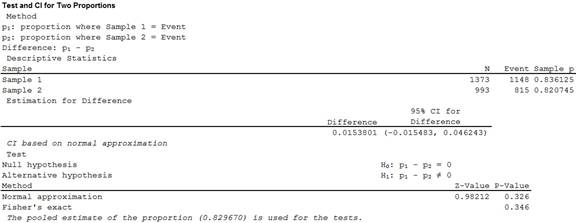
Therefore, the P-value is 0.326.
Hence, it is proved that the P-values for each of these tests are same.
g.
Conclude that when a contingency table has two rows and two columns, the chi square tests equivalent to the test for the difference between proportions.
g.
Explanation of Solution
It is found that the P-values for chi-square test and z test are same. Moreover, the square of z test statistic is same as the chi-square test statistic.
Hence, it can be concluded that when a contingency table has two rows and two columns, the chi square tests equivalent to the test for the difference between proportions.
Want to see more full solutions like this?
Chapter 10 Solutions
ALEKS 360 ESSENT. STAT ACCESS CARD

- Critically analyze the following graph and, based on statistical information, indicate the type of error it presents IN NO MORE THAN 3 LINES SCOTCEN POLL OF POLLS SHOULD SCOTLAND BE INDEPENDENT? NO 52% YES 58% LIVE CAW NAS & 28.30 HAS KILLED MORE THAN 2,600 IN WEST AFRICA, WORLD HEALTH ORG. BROOKEBCNNarrow_forwardCritically analyze the following graph and, based on statistical information, indicate the type of error it presents IN NO MORE THAN 3 LINES PRESIDENTIAL PREFERENCES RODOLFO CARTER 3% (+2pts) EVELYN MATTHEI 22% (+6pts) With the exception of President Boric, could you tell me who you would like to be the next president of Chile? CAMILA VALLEJO 4% (+2pts) JOSÉ ANTONIO KAST 19% (+5pts) MICHELLE BACHELET 6% (+1pts)arrow_forwardCritically analyze the following graph and, based on statistical information, indicate the type of error it presents IN NO MORE THAN 3 LINES 13% APPROVE 4% DOESN'T KNOW DOESN'T RESPOND 5% NEITHER APPROVES NOR DISAPPROVES 78% DISAPPROVES SURVEY PRESIDENTIAL APPROVAL DROPS TO 13%arrow_forward
- Please help with this following question I'm not too sure if question (a) and (b) are correct and not sure how to calculate (c) The csv data is below "","New","Current" "1","67",66 "2","77",73 "3","76",73 "4","76",76 "5","77",79 "6","84",76 "7","71",78 "8","84",72 "9","73",76 "10","71",73 "11","72",77 "12","70",72 "13","75",72 "14","84",71 "15","77",73 "16","65",72 "17","69",73 "18","71",73 "19","79",71 "20","75",78 "21","76",69 "22","73",74 "23","76",71 "24","64",74 "25","81",78 "26","79",76 "27","70",77 "28","79",71 "29","84",73 "30","79",69 "31","69",72 "32","81",76 "33","77",70 "34","77",71 "35","71",69 "36","67",72 "37","70",76 "38","77",73 "39","82",73 "40","72",73arrow_forwardPlease help me answer the following question(c) A previous study found that 15% of nurses reported participating in mental health support programs.From the 96% found in (b) , can you conclude that proportion of nurses reported participating in mental health support programs p(current), has changed from the previous study?(Yes/No) because the confidence interval in (b) (captures/does not capture) 15%.(d) Refer to your answer in (b) : The Alberta Nurses Association expects that not more than 23 % of nurses will participate in the survey on mental health support programs. Given the result in part (b) can we conclude that this expectation is reasonable?(Yes/No) because the (upper bound/lower bound) of the 96% confidence interval is (less than/not less than/greater than) 23%. The Alberta Nursing Association conducts an annual survey to estimate the proportion of nurses who participate in mental health support programs. The most recent application of this survey involved a random sample of…arrow_forwardPlease help me solve this questionThis is what was in the csv file:"","Diabetic","Heart Disease""1",32644,30646"2",789,1670"3",12802,36274"4",2177,5011"5",1910,3300"6",3320,4256"7",61425,39053"8",19768,28635"9",19502,39546"10",5642,12182"11",107864,152098"12",29918,60433"13",2397,3550"14",41559,34705"15",49169,57948"16",72853,83100"17",2155,2873"18",140220,134517"19",28181,26212"20",18850,38637"21",69564,68582"22",13897,12613"23",6868,9138"24",9735,4767"25",12102,13447"26",36571,50010"27",44665,55141"28",26620,33970"29",25525,29766"30",14167,20206Q(b) From this, the relationship between these two variables is (non-existent/positive/negative) . I can categorize this relationship as being (strong/weak/moderate).Q(c) Drop down is (+/-)Q(d) Drop downs in order are __% of the (average/median/variation/standard deviation) in the (the number of people diagnosed with heart disease/the number of people diagnosed with diabetes)−variable can be explained by its (linear relationship/relationship)…arrow_forward
- Please help me answer the following question The drop down for question (e, f, and g) is (YES/NO) Based on the P-value above, the assumption of equal variances among the four machines (Is Met/Is Not Met) Based on the data, the average fill for machine 3 is (statistically lower than/statistically higher than/the same as/not statistically different than/statistically different than/Hard to say then when comparing to/Refuse to say when comparing to) machine 1.arrow_forwardBusiness Discussarrow_forward1 for all k, and set o (ii) Let X1, X2, that P(Xkb) = x > 0. Xn be independent random variables with mean 0, suppose = and Var Xk. Then, for 0x) ≤2 exp-tx+121 Στ k=1arrow_forward
- Lemma 1.1 Suppose that g is a non-negative, non-decreasing function such that E g(X) 0. Then, E g(|X|) P(|X|> x) ≤ g(x)arrow_forwardProof of this Theorem Theorem 1.2 (i) Suppose that P(|X| ≤ b) = 1 for some b > 0, that E X = 0, and set Var X = o². Then, for 0 0, P(X > x) ≤ e−1x+1²², P(|X|> x) ≤ 2e−x+1² 0²arrow_forwardState and prove the Morton's inequality Theorem 1.1 (Markov's inequality) Suppose that E|X|" 0, and let x > 0. Then, E|X|" P(|X|> x) ≤ x"arrow_forward
 MATLAB: An Introduction with ApplicationsStatisticsISBN:9781119256830Author:Amos GilatPublisher:John Wiley & Sons Inc
 Probability and Statistics for Engineering and th...StatisticsISBN:9781305251809Author:Jay L. DevorePublisher:Cengage Learning
 Statistics for The Behavioral Sciences (MindTap C...StatisticsISBN:9781305504912Author:Frederick J Gravetter, Larry B. WallnauPublisher:Cengage Learning
 Elementary Statistics: Picturing the World (7th E...StatisticsISBN:9780134683416Author:Ron Larson, Betsy FarberPublisher:PEARSON
 The Basic Practice of StatisticsStatisticsISBN:9781319042578Author:David S. Moore, William I. Notz, Michael A. FlignerPublisher:W. H. Freeman
 Introduction to the Practice of StatisticsStatisticsISBN:9781319013387Author:David S. Moore, George P. McCabe, Bruce A. CraigPublisher:W. H. Freeman