
Perform test of hypotheses that gender and admission are independent for each department at the level of significance of α=0.01.
Prove that the only department for which this hypothesis is rejected is department A.
Also prove that the admission rate for women in department A is significantly higher than the rate for men.
Answer to Problem 4CS
There is enough evidence to conclude that the gender and admission are not independent of gender in department A.
There is not enough evidence to conclude that the gender and admission are not independent of gender in department B.
There is not enough evidence to conclude that the gender and admission are not independent of gender in department C.
There is not enough evidence to conclude that the gender and admission are not independent of gender in department D.
There is not enough evidence to conclude that the gender and admission are not independent of gender in department E.
There is not enough evidence to conclude that the gender and admission are not independent of gender in department F.
Explanation of Solution
Calculation:
The six contingency tables with 2 rows and 2 columns for each of the six departments are given. The two rows consist of gender and the two columns consist of accepted and rejected applicants.
A contingency table is obtained as using two qualitative variables. One of the qualitative variable is row variable that has one category for each row of the table another is column variable has one category for each column of the table.
Step 1:
For Department A:
The hypotheses are:
Null Hypothesis:
H0:The gender and admission are independent.
Alternate Hypothesis:
H1:The gender and admission are not independent.
Step 2:
Now, it is obtained that,
| Gender | Accept | Reject | Row Total |
| Male | 512 | 313 | 825 |
| Female | 89 | 19 | 108 |
| Column Total | 601 | 332 | 933 |
Step 3:
Expected frequencies:
The expected frequencies in case of contingency table is obtained as,
E=Row total⋅ Coloumn totalGrand total.
Now, using the formula of expected frequency it is found that the expected frequency for the accepted male is obtained as,
(825)(601)933=495,825933=531.430868.
Hence, in similar way the expected frequencies are obtained as,
| Gender | Accept | Reject |
| Male | (825)(601)933=531.430868 | (825)(332)933=293.5691 |
| Female | (108)(601)933=69.5691318 | (108)(332)933=38.43087 |
The accept and reject can be rewritten as,
| Accept | 1 |
| Reject | 2 |
Step 4:
Level of significance:
The level of significance is given as 0.01.
Test Statistic:
Software procedure:
Step -by-step software procedure to obtain test statistic using MINITAB software is as follows:
- Select Stat > Table > Cross Tabulation and Chi-Square.
- Check the box of Raw data (categorical variables).
- Under For rows enter Gender.
- Under For columns enter Column.
- Check the box of Count under Display.
- Under Chi-Square, click the box of Chi-Square test.
- Select OK.
- Output using MINITAB software is given below:
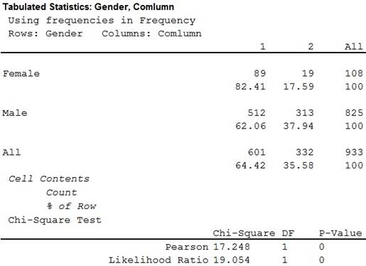
Thus, the value of chi-square statistic is 17.248.
It is known that under the null hypothesis H0 the test statistic χ2=∑(O−E)2E follows chi-square distribution with (r−1)(c−1) degrees of freedom for r number of rows and c number of columns, provided that all the expected frequencies are greater than or equal to 5.
In the given question there are 2 rows and 2 columns.
Hence, the degrees of freedom is
(r−1)(c−1)=(2−1)(2−1)=(1)(1)=1.
Thus, the degrees of freedom is 1.
It is known that when the null hypothesis H0 is true the chi-square statistic for a test of independence, follows approximately chi-square distribution provided that all the expected frequencies are 5 or more.
It is found that all the expected frequencies corresponding to all rows and columns of the given contingency table are more than 5.
Hence, the test of independence is appropriate.
Step 5:
Critical value:
In a test of hypotheses the critical value is the point by which one can reject or accept the null hypothesis.
Software procedure:
Step-by-step software procedure to obtain critical value using MINITAB software is as follows:
- Select Graph > Probability distribution plot > view probability
- Select Chi -Square under distribution.
- In Degrees of freedom, enter 1.
- Choose Probability Value and Right Tail for the region of the curve to shade.
- Enter the Probability value as 0.01 under shaded area.
- Select OK.
- Output using MINITAB software is given below:
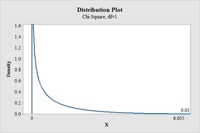
Hence, the critical value at α=0.01 is 6.635.
Rejection rule:
If the χ2 value is greater than or equal to critical value, that is χ2≥χ2α;k−1, then reject the null hypothesis H0. Otherwise, do not reject H0.
Step 6:
Conclusion:
Here, the χ2 value is greater than the critical value.
That is, χ2(=17.248)>χ20.01,1(=6.635)
Thus, the decision is “reject the null hypothesis”.
Thus, there is enough evidence to conclude that the gender and admission are not independent of gender in department A.
For Department B:
Step 1:
The hypotheses are:
The hypotheses are:
Null Hypothesis:
H0:The gender and admission are independent.
Alternate Hypothesis:
H1:The gender and admission are not independent.
Step 2:
Now, it is obtained that,
| Gender | Accept | Reject | Row Total |
| Male | 353 | 207 | 560 |
| Female | 17 | 8 | 25 |
| Column Total | 370 | 215 | 585 |
Step 3:
Now, using the formula of expected frequency it is found that the expected frequency for the accepted male is obtained as,
(560)(370)585=207,200585=354.188034.
Hence, in similar way the expected frequencies are obtained as,
| Gender | Accept | Reject |
| Male | (560)(370)585=354.188034 | (560)(215)585=205.812 |
| Female | (25)(370)585=15.8119658 | (25)(215)585=9.188034 |
The accept and reject can be rewritten as,
| Accept | 1 |
| Reject | 2 |
Step 4:
Level of significance:
The level of significance is given as 0.01.
Test Statistic:
Software procedure:
Step -by-step software procedure to obtain test statistic using MINITAB software is as follows:
- Select Stat > Table > Cross Tabulation and Chi-Square.
- Check the box of Raw data (categorical variables).
- Under For rows enter Gender.
- Under For columns enter Column.
- Check the box of Count under Display.
- Under Chi-Square, click the box of Chi-Square test.
- Select OK.
- Output using MINITAB software is given below:
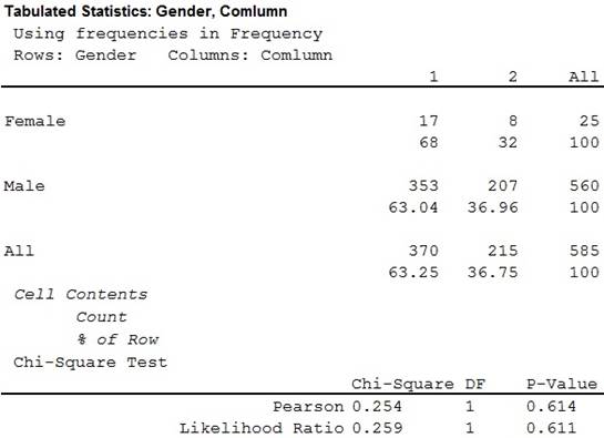
Thus, the value of chi-square statistic is 0.254.
In the given question there are 2 rows and 2 columns.
Hence, the degrees of freedom is
(r−1)(c−1)=(2−1)(2−1)=(1)(1)=1.
Thus, the degrees of freedom is 1.
It is known that when the null hypothesis H0 is true the chi-square statistic for a test of independence, follows approximately chi-square distribution provided that all the expected frequencies are 5 or more.
It is found that all the expected frequencies corresponding to all rows and columns of the given contingency table are more than 5.
Hence, the test of independence is appropriate.
Step 5:
Critical value:
In a test of hypotheses the critical value is the point by which one can reject or accept the null hypothesis.
It is already found that the critical value at α=0.01 is 6.635.
Rejection rule:
If the χ2 value is greater than or equal to critical value, that is χ2≥χ2α;k−1, then reject the null hypothesis H0. Otherwise, do not reject H0.
Step 6:
Conclusion:
Here, the χ2 value is less than the critical value.
That is, χ2(=0.254)<χ20.01,1(=6.635)
Thus, the decision is “fail to reject the null hypothesis”.
Thus, there is not enough evidence to conclude that the gender and admission are not independent of gender in department B.
For Department C:
Step 1:
The hypotheses are:
Null Hypothesis:
H0:The gender and admission are independent.
Alternate Hypothesis:
H1:The gender and admission are not independent.
Step 2:
Now, it is obtained that,
| Gender | Accept | Reject | Row Total |
| Male | 120 | 205 | 325 |
| Female | 202 | 391 | 593 |
| Column Total | 322 | 596 | 918 |
Step 3:
Now, using the formula of expected frequency it is found that the expected frequency for the accepted male is obtained as,
(325)(322)918=104,650918=113.997821.
Hence, in similar way the expected frequencies are obtained as,
| Gender | Accept | Reject |
| Male | (325)(322)918=113.997821 | (325)(596)918=211.0022 |
| Female | (593)(322)918=208.002179 | (593)(596)918=384.9978 |
The accept and reject can be rewritten as,
| Accept | 1 |
| Reject | 2 |
Step 4:
Level of significance:
The level of significance is given as 0.01.
Test Statistic:
Software procedure:
Step -by-step software procedure to obtain test statistic using MINITAB software is as follows:
- Select Stat > Table > Cross Tabulation and Chi-Square.
- Check the box of Raw data (categorical variables).
- Under For rows enter Gender.
- Under For columns enter Column.
- Check the box of Count under Display.
- Under Chi-Square, click the box of Chi-Square test.
- Select OK.
- Output using MINITAB software is given below:
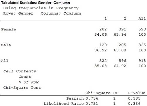
Thus, the value of chi-square statistic is 0.754.
In the given question there are 2 rows and 2 columns.
Hence, the degrees of freedom is
(r−1)(c−1)=(2−1)(2−1)=(1)(1)=1.
Thus, the degrees of freedom is 1.
It is known that when the null hypothesis H0 is true the chi-square statistic for a test of independence, follows approximately chi-square distribution provided that all the expected frequencies are 5 or more.
It is found that all the expected frequencies corresponding to all rows and columns of the given contingency table are more than 5.
Hence, the test of independence is appropriate.
Step 5:
Critical value:
In a test of hypotheses the critical value is the point by which one can reject or accept the null hypothesis.
It is already found that the critical value at α=0.01 is 6.635.
Rejection rule:
If the χ2 value is greater than or equal to critical value, that is χ2≥χ2α;k−1, then reject the null hypothesis H0. Otherwise, do not reject H0.
Step 6:
Conclusion:
Here, the χ2 value is less than the critical value.
That is, χ2(=0.754)<χ20.01,1(=6.635)
Thus, the decision is “fail to reject the null hypothesis”.
Thus, there is not enough evidence to conclude that the gender and admission are not independent of gender in department C.
For Department D:
Step 1:
The hypotheses are:
Null Hypothesis:
H0:The gender and admission are independent.
Alternate Hypothesis:
H1:The gender and admission are not independent.
Step 2:
Now, it is obtained that,
| Gender | Accept | Reject | Row Total |
| Male | 138 | 279 | 417 |
| Female | 131 | 244 | 375 |
| Column Total | 269 | 523 | 792 |
Step 3:
Now, using the formula of expected frequency it is found that the expected frequency for the accepted male is obtained as,
(417)(269)792=112,173792=141.632576.
Hence, in similar way the expected frequencies are obtained as,
| Gender | Accept | Reject |
| Male | (417)(269)792=141.632576 | (417)(523)792=275.3674 |
| Female | (375)(269)792=127.367424 | (375)(523)792=247.6326 |
The accept and reject can be rewritten as,
| Accept | 1 |
| Reject | 2 |
Step 4:
Level of significance:
The level of significance is given as 0.01.
Test Statistic:
Software procedure:
Step -by-step software procedure to obtain test statistic using MINITAB software is as follows:
- Select Stat > Table > Cross Tabulation and Chi-Square.
- Check the box of Raw data (categorical variables).
- Under For rows enter Gender.
- Under For columns enter Column.
- Check the box of Count under Display.
- Under Chi-Square, click the box of Chi-Square test.
- Select OK.
- Output using MINITAB software is given below:
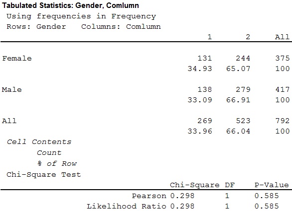
Thus, the value of chi-square statistic is 0.298.
In the given question there are 2 rows and 2 columns.
Hence, the degrees of freedom is
(r−1)(c−1)=(2−1)(2−1)=(1)(1)=1.
Thus, the degrees of freedom is 1.
It is known that when the null hypothesis H0 is true the chi-square statistic for a test of independence, follows approximately chi-square distribution provided that all the expected frequencies are 5 or more.
It is found that all the expected frequencies corresponding to all rows and columns of the given contingency table are more than 5.
Hence, the test of independence is appropriate.
Step 5:
Critical value:
In a test of hypotheses the critical value is the point by which one can reject or accept the null hypothesis.
It is already found that the critical value at α=0.01 is 6.635.
Rejection rule:
If the χ2 value is greater than or equal to critical value, that is χ2≥χ2α;k−1, then reject the null hypothesis H0. Otherwise, do not reject H0.
Step 6:
Conclusion:
Here, the χ2 value is less than the critical value.
That is, χ2(=0.298)<χ20.01,1(=6.635)
Thus, the decision is “fail to reject the null hypothesis”.
Thus, there is not enough evidence to conclude that the gender and admission are not independent of gender in department D.
For Department E:
Step 1:
The hypotheses are:
Null Hypothesis:
H0:The gender and admission are independent.
Alternate Hypothesis:
H1:The gender and admission are not independent.
Step 2:
Now, it is obtained that,
| Gender | Accept | Reject | Row Total |
| Male | 53 | 138 | 191 |
| Female | 94 | 299 | 383 |
| Column Total | 147 | 437 | 584 |
Step 3:
Now, using the formula of expected frequency it is found that the expected frequency for the accepted male is obtained as,
(191)(147)584=28,077584=48.0770548.
Hence, in similar way the expected frequencies are obtained as,
| Gender | Accept | Reject |
| Male | (191)(147)584=48.0770548 | (191)(437)584=142.9229 |
| Female | (383)(147)584=96.40582 | (383)(437)584=286.5941 |
Step 4:
Level of significance:
The level of significance is given as 0.01.
Test Statistic:
Software procedure:
Step -by-step software procedure to obtain test statistic using MINITAB software is as follows:
- Select Stat > Table > Cross Tabulation and Chi-Square.
- Check the box of Raw data (categorical variables).
- Under For rows enter Gender.
- Under For columns enter Column.
- Check the box of Count under Display.
- Under Chi-Square, click the box of Chi-Square test.
- Select OK.
- Output using MINITAB software is given below:
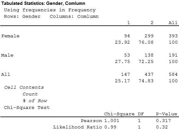
Thus, the value of chi-square statistic is 1.001.
In the given question there are 2 rows and 2 columns.
Hence, the degrees of freedom is
(r−1)(c−1)=(2−1)(2−1)=(1)(1)=1.
Thus, the degrees of freedom is 1.
It is known that when the null hypothesis H0 is true the chi-square statistic for a test of independence, follows approximately chi-square distribution provided that all the expected frequencies are 5 or more.
It is found that all the expected frequencies corresponding to all rows and columns of the given contingency table are more than 5.
Hence, the test of independence is appropriate.
Step 5:
Critical value:
In a test of hypotheses the critical value is the point by which one can reject or accept the null hypothesis.
It is already found that the critical value at α=0.01 is 6.635.
Rejection rule:
If the χ2 value is greater than or equal to critical value, that is χ2≥χ2α;k−1, then reject the null hypothesis H0. Otherwise, do not reject H0.
Step 6:
Conclusion:
Here, the χ2 value is less than the critical value.
That is, χ2(=1.001)<χ20.01,1(=6.635)
Thus, the decision is “fail to reject the null hypothesis”.
Thus, there is not enough evidence to conclude that the gender and admission are not independent of gender in department E.
For Department F:
Step 1:
The hypotheses are:
Null Hypothesis:
H0:The gender and admission are independent.
Alternate Hypothesis:
H1:The gender and admission are not independent.
Step 2:
Now, it is obtained that,
| Gender | Accept | Reject | Row Total |
| Male | 22 | 351 | 373 |
| Female | 24 | 317 | 341 |
| Column Total | 46 | 668 | 714 |
Step 3:
Now, using the formula of expected frequency it is found that the expected frequency for the accepted male is obtained as,
(373)(46)714=17,158714=24.0308123.
Hence, in similar way the expected frequencies are obtained as,
| Gender | Accept | Reject |
| Male | (373)(46)714=24.0308123 | (373)(668)714=348.9692 |
| Female | (341)(46)714=21.9691877 | (341)(668)714=319.0308 |
The accept and reject can be rewritten as,
| Accept | 1 |
| Reject | 2 |
Step 4:
Level of significance:
The level of significance is given as 0.01.
Test Statistic:
Software procedure:
Step -by-step software procedure to obtain test statistic using MINITAB software is as follows:
- Select Stat > Table > Cross Tabulation and Chi-Square.
- Check the box of Raw data (categorical variables).
- Under For rows enter Gender.
- Under For columns enter Column.
- Check the box of Count under Display.
- Under Chi-Square, click the box of Chi-Square test.
- Select OK.
- Output using MINITAB software is given below:
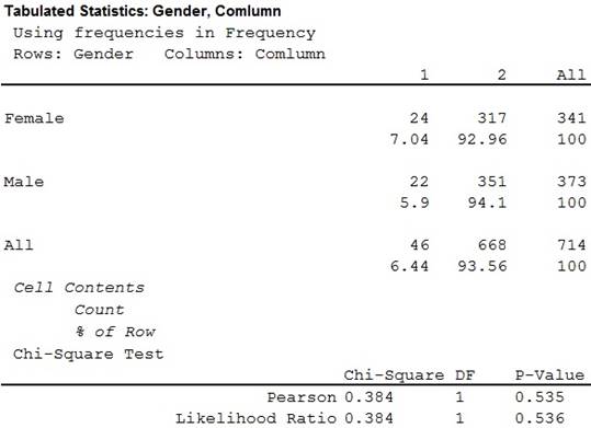
Thus, the value of chi-square statistic is 0.384.
In the given question there are 2 rows and 2 columns.
Hence, the degrees of freedom is
(r−1)(c−1)=(2−1)(2−1)=(1)(1)=1.
Thus, the degrees of freedom is 1.
It is known that when the null hypothesis H0 is true the chi-square statistic for a test of independence, follows approximately chi-square distribution provided that all the expected frequencies are 5 or more.
It is found that all the expected frequencies corresponding to all rows and columns of the given contingency table are more than 5.
Hence, the test of independence is appropriate.
Step 5:
Critical value:
In a test of hypotheses the critical value is the point by which one can reject or accept the null hypothesis.
It is already found that the critical value at α=0.01 is 6.635.
Rejection rule:
If the χ2 value is greater than or equal to critical value, that is χ2≥χ2α;k−1, then reject the null hypothesis H0. Otherwise, do not reject H0.
Step 6:
Conclusion:
Here, the χ2 value is less than the critical value.
That is, χ2(=0.384)<χ20.01,1(=6.635)
Thus, the decision is “fail to reject the null hypothesis”.
Thus, there is not enough evidence to conclude that the gender and admission are not independent of gender in department F.
Thus, it is clear that the only department for which this hypothesis is rejected is department A.
The accepted number of women out of total 108 women is 89.
Hence, the percentage of accepted number of women in department A is,
89108×100%=82.4%.
The accepted number of men out of total 825 men is 512.
Hence, the accepted number of men in department A is,
512825×100%=62.06%.
Thus, it can be concluded that the admission rate for women in department A is significantly higher than the rate for men.
Want to see more full solutions like this?
Chapter 10 Solutions
ALEKS 360 ESSENT. STAT ACCESS CARD

- ons 12. A sociologist hypothesizes that the crime rate is higher in areas with higher poverty rate and lower median income. She col- lects data on the crime rate (crimes per 100,000 residents), the poverty rate (in %), and the median income (in $1,000s) from 41 New England cities. A portion of the regression results is shown in the following table. Standard Coefficients error t stat p-value Intercept -301.62 549.71 -0.55 0.5864 Poverty 53.16 14.22 3.74 0.0006 Income 4.95 8.26 0.60 0.5526 a. b. Are the signs as expected on the slope coefficients? Predict the crime rate in an area with a poverty rate of 20% and a median income of $50,000. 3. Using data from 50 workarrow_forward2. The owner of several used-car dealerships believes that the selling price of a used car can best be predicted using the car's age. He uses data on the recent selling price (in $) and age of 20 used sedans to estimate Price = Po + B₁Age + ε. A portion of the regression results is shown in the accompanying table. Standard Coefficients Intercept 21187.94 Error 733.42 t Stat p-value 28.89 1.56E-16 Age -1208.25 128.95 -9.37 2.41E-08 a. What is the estimate for B₁? Interpret this value. b. What is the sample regression equation? C. Predict the selling price of a 5-year-old sedan.arrow_forwardian income of $50,000. erty rate of 13. Using data from 50 workers, a researcher estimates Wage = Bo+B,Education + B₂Experience + B3Age+e, where Wage is the hourly wage rate and Education, Experience, and Age are the years of higher education, the years of experience, and the age of the worker, respectively. A portion of the regression results is shown in the following table. ni ogolloo bash 1 Standard Coefficients error t stat p-value Intercept 7.87 4.09 1.93 0.0603 Education 1.44 0.34 4.24 0.0001 Experience 0.45 0.14 3.16 0.0028 Age -0.01 0.08 -0.14 0.8920 a. Interpret the estimated coefficients for Education and Experience. b. Predict the hourly wage rate for a 30-year-old worker with four years of higher education and three years of experience.arrow_forward
- 1. If a firm spends more on advertising, is it likely to increase sales? Data on annual sales (in $100,000s) and advertising expenditures (in $10,000s) were collected for 20 firms in order to estimate the model Sales = Po + B₁Advertising + ε. A portion of the regression results is shown in the accompanying table. Intercept Advertising Standard Coefficients Error t Stat p-value -7.42 1.46 -5.09 7.66E-05 0.42 0.05 8.70 7.26E-08 a. Interpret the estimated slope coefficient. b. What is the sample regression equation? C. Predict the sales for a firm that spends $500,000 annually on advertising.arrow_forwardCan you help me solve problem 38 with steps im stuck.arrow_forwardHow do the samples hold up to the efficiency test? What percentages of the samples pass or fail the test? What would be the likelihood of having the following specific number of efficiency test failures in the next 300 processors tested? 1 failures, 5 failures, 10 failures and 20 failures.arrow_forward
- The battery temperatures are a major concern for us. Can you analyze and describe the sample data? What are the average and median temperatures? How much variability is there in the temperatures? Is there anything that stands out? Our engineers’ assumption is that the temperature data is normally distributed. If that is the case, what would be the likelihood that the Safety Zone temperature will exceed 5.15 degrees? What is the probability that the Safety Zone temperature will be less than 4.65 degrees? What is the actual percentage of samples that exceed 5.25 degrees or are less than 4.75 degrees? Is the manufacturing process producing units with stable Safety Zone temperatures? Can you check if there are any apparent changes in the temperature pattern? Are there any outliers? A closer look at the Z-scores should help you in this regard.arrow_forwardNeed help pleasearrow_forwardPlease conduct a step by step of these statistical tests on separate sheets of Microsoft Excel. If the calculations in Microsoft Excel are incorrect, the null and alternative hypotheses, as well as the conclusions drawn from them, will be meaningless and will not receive any points. 4. One-Way ANOVA: Analyze the customer satisfaction scores across four different product categories to determine if there is a significant difference in means. (Hints: The null can be about maintaining status-quo or no difference among groups) H0 = H1=arrow_forward
- Please conduct a step by step of these statistical tests on separate sheets of Microsoft Excel. If the calculations in Microsoft Excel are incorrect, the null and alternative hypotheses, as well as the conclusions drawn from them, will be meaningless and will not receive any points 2. Two-Sample T-Test: Compare the average sales revenue of two different regions to determine if there is a significant difference. (Hints: The null can be about maintaining status-quo or no difference among groups; if alternative hypothesis is non-directional use the two-tailed p-value from excel file to make a decision about rejecting or not rejecting null) H0 = H1=arrow_forwardPlease conduct a step by step of these statistical tests on separate sheets of Microsoft Excel. If the calculations in Microsoft Excel are incorrect, the null and alternative hypotheses, as well as the conclusions drawn from them, will be meaningless and will not receive any points 3. Paired T-Test: A company implemented a training program to improve employee performance. To evaluate the effectiveness of the program, the company recorded the test scores of 25 employees before and after the training. Determine if the training program is effective in terms of scores of participants before and after the training. (Hints: The null can be about maintaining status-quo or no difference among groups; if alternative hypothesis is non-directional, use the two-tailed p-value from excel file to make a decision about rejecting or not rejecting the null) H0 = H1= Conclusion:arrow_forwardPlease conduct a step by step of these statistical tests on separate sheets of Microsoft Excel. If the calculations in Microsoft Excel are incorrect, the null and alternative hypotheses, as well as the conclusions drawn from them, will be meaningless and will not receive any points. The data for the following questions is provided in Microsoft Excel file on 4 separate sheets. Please conduct these statistical tests on separate sheets of Microsoft Excel. If the calculations in Microsoft Excel are incorrect, the null and alternative hypotheses, as well as the conclusions drawn from them, will be meaningless and will not receive any points. 1. One Sample T-Test: Determine whether the average satisfaction rating of customers for a product is significantly different from a hypothetical mean of 75. (Hints: The null can be about maintaining status-quo or no difference; If your alternative hypothesis is non-directional (e.g., μ≠75), you should use the two-tailed p-value from excel file to…arrow_forward
 MATLAB: An Introduction with ApplicationsStatisticsISBN:9781119256830Author:Amos GilatPublisher:John Wiley & Sons Inc
 Probability and Statistics for Engineering and th...StatisticsISBN:9781305251809Author:Jay L. DevorePublisher:Cengage Learning
 Statistics for The Behavioral Sciences (MindTap C...StatisticsISBN:9781305504912Author:Frederick J Gravetter, Larry B. WallnauPublisher:Cengage Learning
 Elementary Statistics: Picturing the World (7th E...StatisticsISBN:9780134683416Author:Ron Larson, Betsy FarberPublisher:PEARSON
 The Basic Practice of StatisticsStatisticsISBN:9781319042578Author:David S. Moore, William I. Notz, Michael A. FlignerPublisher:W. H. Freeman
 Introduction to the Practice of StatisticsStatisticsISBN:9781319013387Author:David S. Moore, George P. McCabe, Bruce A. CraigPublisher:W. H. Freeman