Concept explainers
Videos
The range of values of P for which the equilibrium of the system is stable.
Answer to Problem 10.98P
The range of values of P for which the equilibrium position is stable is
Explanation of Solution
Given information:
The system is in equilibrium when
The length of the bars AB and BC is
The spring constant is
Calculation:
Draw the free-body diagram of the arrangement as in Figure (1).
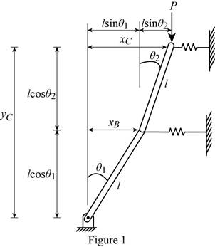
Find the horizontal distance
Find the horizontal distance
Find the vertical distance
When the values are small,
Find the potential energy (V) using the relation.
Here, the magnitude of the force applied at C is P and the spring constant is k.
Substitute
Substitute
Differentiate the Equation (1) with respect to
Differentiate the Equation (2).
Differentiate the equation (2) with
Differentiate the Equation (1) with respect to
Differentiate the Equation;
Condition 1:
When the equilibrium is stable,
Substitute 0 for
Substitute 0 for
The condition is satisfied. The equilibrium is stable.
Condition 2:
Check the condition,
Substitute
Solve the equation using the mathematical equation.
Condition 3;
Check the condition;
Condition 4:
Refer to all the conditions,
The minimum value of P is 0.
The maximum value of P is
Substitute
Thus, the range of values of P for which the equilibrium position is stable is
Want to see more full solutions like this?
Chapter 10 Solutions
Vector Mechanics for Engineers: Statics and Dynamics


- PROBLEM 3.46 The solid cylindrical rod BC of length L = 600 mm is attached to the rigid lever AB of length a = 380 mm and to the support at C. When a 500 N force P is applied at A, design specifications require that the displacement of A not exceed 25 mm when a 500 N force P is applied at A For the material indicated determine the required diameter of the rod. Aluminium: Tall = 65 MPa, G = 27 GPa. Aarrow_forwardFind the equivalent mass of the rocker arm assembly with respect to the x coordinate. k₁ mi m2 k₁arrow_forward2. Figure below shows a U-tube manometer open at both ends and containing a column of liquid mercury of length l and specific weight y. Considering a small displacement x of the manometer meniscus from its equilibrium position (or datum), determine the equivalent spring constant associated with the restoring force. Datum Area, Aarrow_forward
- 1. The consequences of a head-on collision of two automobiles can be studied by considering the impact of the automobile on a barrier, as shown in figure below. Construct a mathematical model (i.e., draw the diagram) by considering the masses of the automobile body, engine, transmission, and suspension and the elasticity of the bumpers, radiator, sheet metal body, driveline, and engine mounts.arrow_forward3.) 15.40 – Collar B moves up at constant velocity vB = 1.5 m/s. Rod AB has length = 1.2 m. The incline is at angle = 25°. Compute an expression for the angular velocity of rod AB, ė and the velocity of end A of the rod (✓✓) as a function of v₂,1,0,0. Then compute numerical answers for ȧ & y_ with 0 = 50°.arrow_forward2.) 15.12 The assembly shown consists of the straight rod ABC which passes through and is welded to the grectangular plate DEFH. The assembly rotates about the axis AC with a constant angular velocity of 9 rad/s. Knowing that the motion when viewed from C is counterclockwise, determine the velocity and acceleration of corner F.arrow_forward
 Elements Of ElectromagneticsMechanical EngineeringISBN:9780190698614Author:Sadiku, Matthew N. O.Publisher:Oxford University Press
 Mechanics of Materials (10th Edition)Mechanical EngineeringISBN:9780134319650Author:Russell C. HibbelerPublisher:PEARSON
 Thermodynamics: An Engineering ApproachMechanical EngineeringISBN:9781259822674Author:Yunus A. Cengel Dr., Michael A. BolesPublisher:McGraw-Hill Education
 Control Systems EngineeringMechanical EngineeringISBN:9781118170519Author:Norman S. NisePublisher:WILEY
 Mechanics of Materials (MindTap Course List)Mechanical EngineeringISBN:9781337093347Author:Barry J. Goodno, James M. GerePublisher:Cengage Learning
 Engineering Mechanics: StaticsMechanical EngineeringISBN:9781118807330Author:James L. Meriam, L. G. Kraige, J. N. BoltonPublisher:WILEY