
Concept explainers
Videos
Anorexia again Refer to Exercise 10.89, comparing
MINITAB output for comparing mean weight changes
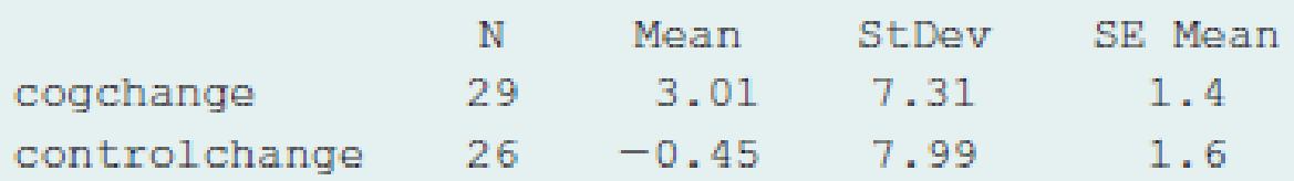
Difference = μ(cogchange) − μ(controlchange)
Estimate for difference: 3.46
95% CI for difference:(−0.68, 7.59)
T-Test of difference = 0 (vs ≠):
T-Value = 1.68 P-Value = 0.100 DF = 53
Both use Pooled StDev = 7.6369
- a. Interpret the reported confidence interval.
- b. Interpret the reported P-value.
- c. What would be the P-value for Ha: μ1 > μ2? Interpret it.
- d. What assumptions do these inferences make?
Teenage anorexia Example 8 in Section 9.3 described a study that used a cognitive behavioral therapy to treat a sample of teenage girls who suffered from anorexia. The study observed the mean weight change after a period of treatment. Studies of that type also usually have a control group that receives no treatment or a standard treatment. Then researchers can analyze how the change in weight compares for the treatment group to the control group. In fact, the anorexia study had a control group that received a standard treatment. Teenage girls in the study were randomly assigned to the cognitive behavioral treatment (Group 1) or to the control group (Group 2). The figure shows box plots of the weight changes for the two groups (displayed vertically). The output shows how MINITAB reports inferential comparisons of those two means.
MINITAB Output Comparing Mean Weight Changes
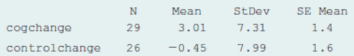
Difference = μ(cogchange) − μ(controlchange)
Estimate for difference: 3.46
95% CI for difference: (−0.71, 7.62)
T-Test of difference = 0 (vs ≠):
T-Value = 1.67 P-Value = 0.102 DF = 50
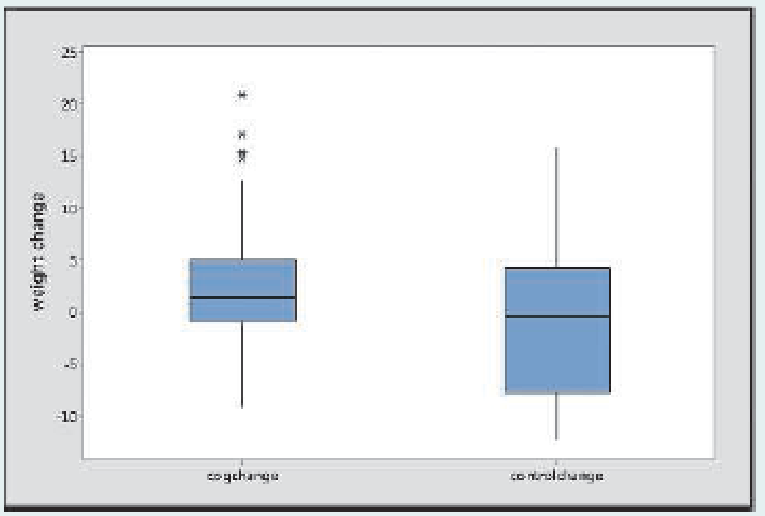
Box plots of weight change for anorexia study.
- a. Report and interpret the P-value for testing H0: μ1 = μ2 against Ha: μ1 ≠∙ μ2.
- b. Summarize the assumptions needed for the analysis in part a. Based on the box plots, would you be nervous if you had to perform a one-sided test instead? Why?
- c. The reported 95% confidence interval tells us that if the population mean weight change is less for the cognitive behavioral group than for the control group, it is just barely less (less than 1 pound), but if the population mean change is greater, it could be nearly 8 pounds greater. Explain how to get this interpretation from the interval reported.
- d. Explain the correspondence between the confidence interval and the decision in the significance test for a 0.05 significance level.
Want to see the full answer?
Check out a sample textbook solution
Chapter 10 Solutions
Statistics: The Art and Science of Learning from Data (4th Edition)


- 21. ANALYSIS OF LAST DIGITS Heights of statistics students were obtained by the author as part of an experiment conducted for class. The last digits of those heights are listed below. Construct a frequency distribution with 10 classes. Based on the distribution, do the heights appear to be reported or actually measured? Does there appear to be a gap in the frequencies and, if so, how might that gap be explained? What do you know about the accuracy of the results? 3 4 555 0 0 0 0 0 0 0 0 0 1 1 23 3 5 5 5 5 5 5 5 5 5 5 5 5 6 6 8 8 8 9arrow_forwardA side view of a recycling bin lid is diagramed below where two panels come together at a right angle. 45 in 24 in Width? — Given this information, how wide is the recycling bin in inches?arrow_forward1 No. 2 3 4 Binomial Prob. X n P Answer 5 6 4 7 8 9 10 12345678 8 3 4 2 2552 10 0.7 0.233 0.3 0.132 7 0.6 0.290 20 0.02 0.053 150 1000 0.15 0.035 8 7 10 0.7 0.383 11 9 3 5 0.3 0.132 12 10 4 7 0.6 0.290 13 Poisson Probability 14 X lambda Answer 18 4 19 20 21 22 23 9 15 16 17 3 1234567829 3 2 0.180 2 1.5 0.251 12 10 0.095 5 3 0.101 7 4 0.060 3 2 0.180 2 1.5 0.251 24 10 12 10 0.095arrow_forward
- step by step on Microssoft on how to put this in excel and the answers please Find binomial probability if: x = 8, n = 10, p = 0.7 x= 3, n=5, p = 0.3 x = 4, n=7, p = 0.6 Quality Control: A factory produces light bulbs with a 2% defect rate. If a random sample of 20 bulbs is tested, what is the probability that exactly 2 bulbs are defective? (hint: p=2% or 0.02; x =2, n=20; use the same logic for the following problems) Marketing Campaign: A marketing company sends out 1,000 promotional emails. The probability of any email being opened is 0.15. What is the probability that exactly 150 emails will be opened? (hint: total emails or n=1000, x =150) Customer Satisfaction: A survey shows that 70% of customers are satisfied with a new product. Out of 10 randomly selected customers, what is the probability that at least 8 are satisfied? (hint: One of the keyword in this question is “at least 8”, it is not “exactly 8”, the correct formula for this should be = 1- (binom.dist(7, 10, 0.7,…arrow_forwardKate, Luke, Mary and Nancy are sharing a cake. The cake had previously been divided into four slices (s1, s2, s3 and s4). What is an example of fair division of the cake S1 S2 S3 S4 Kate $4.00 $6.00 $6.00 $4.00 Luke $5.30 $5.00 $5.25 $5.45 Mary $4.25 $4.50 $3.50 $3.75 Nancy $6.00 $4.00 $4.00 $6.00arrow_forwardFaye cuts the sandwich in two fair shares to her. What is the first half s1arrow_forward
- Question 2. An American option on a stock has payoff given by F = f(St) when it is exercised at time t. We know that the function f is convex. A person claims that because of convexity, it is optimal to exercise at expiration T. Do you agree with them?arrow_forwardQuestion 4. We consider a CRR model with So == 5 and up and down factors u = 1.03 and d = 0.96. We consider the interest rate r = 4% (over one period). Is this a suitable CRR model? (Explain your answer.)arrow_forwardQuestion 3. We want to price a put option with strike price K and expiration T. Two financial advisors estimate the parameters with two different statistical methods: they obtain the same return rate μ, the same volatility σ, but the first advisor has interest r₁ and the second advisor has interest rate r2 (r1>r2). They both use a CRR model with the same number of periods to price the option. Which advisor will get the larger price? (Explain your answer.)arrow_forward
- Question 5. We consider a put option with strike price K and expiration T. This option is priced using a 1-period CRR model. We consider r > 0, and σ > 0 very large. What is the approximate price of the option? In other words, what is the limit of the price of the option as σ∞. (Briefly justify your answer.)arrow_forwardQuestion 6. You collect daily data for the stock of a company Z over the past 4 months (i.e. 80 days) and calculate the log-returns (yk)/(-1. You want to build a CRR model for the evolution of the stock. The expected value and standard deviation of the log-returns are y = 0.06 and Sy 0.1. The money market interest rate is r = 0.04. Determine the risk-neutral probability of the model.arrow_forwardSeveral markets (Japan, Switzerland) introduced negative interest rates on their money market. In this problem, we will consider an annual interest rate r < 0. We consider a stock modeled by an N-period CRR model where each period is 1 year (At = 1) and the up and down factors are u and d. (a) We consider an American put option with strike price K and expiration T. Prove that if <0, the optimal strategy is to wait until expiration T to exercise.arrow_forward
 Glencoe Algebra 1, Student Edition, 9780079039897...AlgebraISBN:9780079039897Author:CarterPublisher:McGraw Hill
 Big Ideas Math A Bridge To Success Algebra 1: Stu...AlgebraISBN:9781680331141Author:HOUGHTON MIFFLIN HARCOURTPublisher:Houghton Mifflin Harcourt