
Fluid Mechanics: Fundamentals and Applications
4th Edition
ISBN: 9781259877827
Author: CENGEL
Publisher: MCG
expand_more
expand_more
format_list_bulleted
Concept explainers
Videos
Textbook Question
Chapter 10, Problem 51CP
Consider the flow field produced by a hair dayer (Fig. P10-51C). Identify regions of this flow field that can be approximated as irrotational, and those for the irrotational flow approximationwould not be appropriate (rotational flow regions).
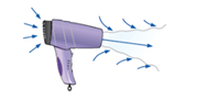
FIGURE P10-51C
Expert Solution & Answer
Want to see the full answer?
Check out a sample textbook solution
Students have asked these similar questions
The 2-mass system shown below depicts a disk which rotates about its center and has rotational
moment of inertia Jo and radius r. The angular displacement of the disk is given by 0. The spring
with constant k₂ is attached to the disk at a distance from the center. The mass m has linear
displacement & and is subject to an external force u. When the system is at equilibrium, the spring
forces due to k₁ and k₂ are zero. Neglect gravity and aerodynamic drag in this problem. You may
assume the small angle approximation which implies (i) that the springs and dampers remain in
their horizontal / vertical configurations and (ii) that the linear displacement d of a point on the
edge of the disk can be approximated by d≈re.
Ө
K2
www
m
4
Cz
777777
Jo
Make the following assumptions when analyzing the forces and torques:
тв
2
0>0, 0>0, x> > 0, >0
Derive the differential equations of motion for this dynamic system. Start by sketching
LARGE and carefully drawn free-body-diagrams for the disk and the…
A linear system is one that satisfies the principle of superposition. In other words, if an input u₁
yields the output y₁, and an input u2 yields the output y2, the system is said to be linear if a com-
bination of the inputs u = u₁ + u2 yield the sum of the outputs y = y1 + y2.
Using this fact, determine the output y(t) of the following linear system:
given the input:
P(s) =
=
Y(s)
U(s)
=
s+1
s+10
u(t) = e−2+ sin(t)
=e
The manometer fluid in the figure given below is mercury where D = 3 in and h = 1 in. Estimate the volume flow in the tube (ft3/s) if the flowing fluid is gasoline at 20°C and 1 atm. The density of mercury and gasoline are 26.34 slug/ft3 and 1.32 slug/ft3 respectively. The gravitational force is 32.2 ft/s2.
Chapter 10 Solutions
Fluid Mechanics: Fundamentals and Applications
Ch. 10 - Discuss how nondimensalizsionalization of the...Ch. 10 - Prob. 2CPCh. 10 - Expalain the difference between an “exact”...Ch. 10 - Prob. 4CPCh. 10 - Prob. 5CPCh. 10 - Prob. 6CPCh. 10 - Prob. 7CPCh. 10 - A box fan sits on the floor of a very large room...Ch. 10 - Prob. 9PCh. 10 - Prob. 10P
Ch. 10 - Prob. 11PCh. 10 - In Example 9-18 we solved the Navier-Stekes...Ch. 10 - Prob. 13PCh. 10 - A flow field is simulated by a computational fluid...Ch. 10 - In Chap. 9(Example 9-15), we generated an “exact”...Ch. 10 - Prob. 16CPCh. 10 - Prob. 17CPCh. 10 - A person drops 3 aluminum balls of diameters 2 mm,...Ch. 10 - Prob. 19PCh. 10 - Prob. 20PCh. 10 - Prob. 21PCh. 10 - Prob. 22PCh. 10 - Prob. 23PCh. 10 - Prob. 24PCh. 10 - Prob. 25PCh. 10 - Prob. 26PCh. 10 - Prob. 27PCh. 10 - Consider again the slipper-pad bearing of Prob....Ch. 10 - Consider again the slipper the slipper-pad bearing...Ch. 10 - Prob. 30PCh. 10 - Prob. 31PCh. 10 - Prob. 32PCh. 10 - Prob. 33PCh. 10 - Prob. 34EPCh. 10 - Discuss what happens when oil temperature...Ch. 10 - Prob. 36PCh. 10 - Prob. 38PCh. 10 - Prob. 39CPCh. 10 - Prob. 40CPCh. 10 - Prob. 41PCh. 10 - Prob. 42PCh. 10 - Prob. 43PCh. 10 - Prob. 44PCh. 10 - Prob. 45PCh. 10 - Prob. 46PCh. 10 - Prob. 47PCh. 10 - Prob. 48PCh. 10 -
Ch. 10 - Prob. 50CPCh. 10 - Consider the flow field produced by a hair dayer...Ch. 10 - In an irrotational region of flow, the velocity...Ch. 10 -
Ch. 10 - Prob. 54CPCh. 10 - Prob. 55PCh. 10 - Prob. 56PCh. 10 - Consider the following steady, two-dimensional,...Ch. 10 - Prob. 58PCh. 10 - Consider the following steady, two-dimensional,...Ch. 10 - Prob. 60PCh. 10 - Consider a steady, two-dimensional,...Ch. 10 -
Ch. 10 - Prob. 63PCh. 10 - Prob. 64PCh. 10 - Prob. 65PCh. 10 - In an irrotational region of flow, we wtite the...Ch. 10 - Prob. 67PCh. 10 - Prob. 68PCh. 10 - Water at atmospheric pressure and temperature...Ch. 10 - The stream function for steady, incompressible,...Ch. 10 -
Ch. 10 - We usually think of boundary layers as occurring...Ch. 10 - Prob. 73CPCh. 10 - Prob. 74CPCh. 10 - Prob. 75CPCh. 10 - Prob. 76CPCh. 10 - Prob. 77CPCh. 10 - Prob. 78CPCh. 10 - Prob. 79CPCh. 10 - Prob. 80CPCh. 10 - Prob. 81CPCh. 10 -
Ch. 10 - On a hot day (T=30C) , a truck moves along the...Ch. 10 - A boat moves through water (T=40F) .18.0 mi/h. A...Ch. 10 - Air flows parallel to a speed limit sign along the...Ch. 10 - Air flows through the test section of a small wind...Ch. 10 - Prob. 87EPCh. 10 - Consider the Blasius solution for a laminar flat...Ch. 10 - Prob. 89PCh. 10 - A laminar flow wind tunnel has a test is 30cm in...Ch. 10 - Repeat the calculation of Prob. 10-90, except for...Ch. 10 - Prob. 92PCh. 10 - Prob. 93EPCh. 10 - Prob. 94EPCh. 10 - In order to avoid boundary laver interference,...Ch. 10 - The stramwise velocity component of steady,...Ch. 10 - For the linear approximation of Prob. 10-97, use...Ch. 10 - Prob. 99PCh. 10 - One dimension of a rectangular fiat place is twice...Ch. 10 - Prob. 101PCh. 10 - Prob. 102PCh. 10 - Prob. 103PCh. 10 - Static pressure P is measured at two locations...Ch. 10 - Prob. 105PCh. 10 - For each statement, choose whether the statement...Ch. 10 - Prob. 107PCh. 10 - Calculate the nine components of the viscous...Ch. 10 - In this chapter, we discuss the line vortex (Fig....Ch. 10 - Calculate the nine components of the viscous...Ch. 10 - Prob. 111PCh. 10 - The streamwise velocity component of a steady...Ch. 10 - For the sine wave approximation of Prob. 10-112,...Ch. 10 - Prob. 115PCh. 10 - Suppose the vertical pipe of prob. 10-115 is now...Ch. 10 - Which choice is not a scaling parameter used to o...Ch. 10 - Prob. 118PCh. 10 - Which dimensionless parameter does not appear m...Ch. 10 - Prob. 120PCh. 10 - Prob. 121PCh. 10 - Prob. 122PCh. 10 - Prob. 123PCh. 10 - Prob. 124PCh. 10 - Prob. 125PCh. 10 - Prob. 126PCh. 10 - Prob. 127PCh. 10 - Prob. 128PCh. 10 - Prob. 129PCh. 10 - Prob. 130PCh. 10 - Prob. 131PCh. 10 - Prob. 132PCh. 10 - Prob. 133PCh. 10 - Prob. 134PCh. 10 - Prob. 135PCh. 10 - Prob. 136PCh. 10 - Prob. 137PCh. 10 - Prob. 138P
Knowledge Booster


Learn more about
Need a deep-dive on the concept behind this application? Look no further. Learn more about this topic, mechanical-engineering and related others by exploring similar questions and additional content below.Similar questions
- Using the Bernoulli equation to find the general solution. If an initial condition is given, find the particular solution. y' + xy = xy¯¹, y(0) = 3arrow_forwardTest for exactness. If exact, solve. If not, use an integrating factor as given or obtained by inspection or by the theorems in the text. a. 2xydx+x²dy = 0 b. (x2+y2)dx-2xydy = 0 c. 6xydx+5(y + x2)dy = 0arrow_forwardNewton's law of cooling. A thermometer, reading 5°C, is brought into a room whose temperature is 22°C. One minute later the thermometer reading is 12°C. How long does it take until the reading is practically 22°C, say, 21.9°C?arrow_forward
- Solve a. y' + 2xy = ex-x² b. y' + y sin x = ecosx, y(0) = −1 y(0) = −2.5arrow_forward= MMB 241 Tutorial 3.pdf 2/6 90% + + 5. The boat is traveling along the circular path with a speed of v = (0.0625t²) m/s, where t is in seconds. Determine the magnitude of its acceleration when t = 10 s. 40 m v = 0.0625² 6. If the motorcycle has a deceleration of at = (0.001s) m/s² and its speed at position A is 25 m/s, determine the magnitude of its acceleration when it passes point B. .A 90° 300 m n B 2arrow_forward= MMB 241 Tutorial 3.pdf 4/6 67% + 9. The car is traveling along the road with a speed of v = (2 s) m/s, where s is in meters. Determine the magnitude of its acceleration when s = 10 m. v = (2s) m/s 50 m 10. The platform is rotating about the vertical axis such that at any instant its angular position is u = (4t 3/2) rad, where t is in seconds. A ball rolls outward along the radial groove so that its position is r = (0.1+³) m, where t is in seconds. Determine the magnitudes of the velocity and acceleration of the ball when t = 1.5s.arrow_forward
- The population of a certain country is known to increase at a rate proportional to the number of people presently living in the country. If after two years the population has doubled, and after three years the population is 20,000, estimate the number of people initially living in the country.arrow_forward= MMB 241 Tutorial 3.pdf 6/6 100% + | 日 13. The slotted link is pinned at O, and as a result of the constant angular velocity *= 3 rad/s it drives the peg P for a short distance along the spiral guide r = (0.40) m, where 0 is in radians. Determine the radial and transverse components of the velocity and acceleration of P at the instant = 1/3 rad. 0.5 m P r = 0.40 =3 rad/sarrow_forward= MMB 241 Tutorial 3.pdf 1/6 90% + DYNAMICS OF PARTICLES (MMB 241) Tutorial 3 Topic: Kinematics of Particles:- Path and Polar coordinate systems and general curvilinear QUESTIONS motion. 1. Determine the acceleration at s = 2 m if v = (2 s) m/s², where s is in meters. At s = 0, v = 1 m/s. 3 m 2. Determine the acceleration when t=1s if v = (4t2+2) m/s, where t is in seconds. v=(4²+2) m/s 6 marrow_forward
- 5.112 A mounting bracket for electronic components is formed from sheet metal with a uniform thickness. Locate the center of gravity of the bracket. 0.75 in. 3 in. ༧ Fig. P5.112 1.25 in. 0.75 in. y r = 0.625 in. 2.5 in. 1 in. 6 in. xarrow_forward4-105. Replace the force system acting on the beam by an equivalent resultant force and couple moment at point B. A 30 in. 4 in. 12 in. 16 in. B 30% 3 in. 10 in. 250 lb 260 lb 13 5 12 300 lbarrow_forwardSketch and Describe a hatch coaming and show how the hatch coamings are framed in to ships strucure?arrow_forward
arrow_back_ios
SEE MORE QUESTIONS
arrow_forward_ios
Recommended textbooks for you
 Elements Of ElectromagneticsMechanical EngineeringISBN:9780190698614Author:Sadiku, Matthew N. O.Publisher:Oxford University Press
 Mechanics of Materials (10th Edition)Mechanical EngineeringISBN:9780134319650Author:Russell C. HibbelerPublisher:PEARSON
 Thermodynamics: An Engineering ApproachMechanical EngineeringISBN:9781259822674Author:Yunus A. Cengel Dr., Michael A. BolesPublisher:McGraw-Hill Education
 Control Systems EngineeringMechanical EngineeringISBN:9781118170519Author:Norman S. NisePublisher:WILEY
 Mechanics of Materials (MindTap Course List)Mechanical EngineeringISBN:9781337093347Author:Barry J. Goodno, James M. GerePublisher:Cengage Learning
 Engineering Mechanics: StaticsMechanical EngineeringISBN:9781118807330Author:James L. Meriam, L. G. Kraige, J. N. BoltonPublisher:WILEY
Elements Of Electromagnetics
Mechanical Engineering
ISBN:9780190698614
Author:Sadiku, Matthew N. O.
Publisher:Oxford University Press
Mechanics of Materials (10th Edition)
Mechanical Engineering
ISBN:9780134319650
Author:Russell C. Hibbeler
Publisher:PEARSON
Thermodynamics: An Engineering Approach
Mechanical Engineering
ISBN:9781259822674
Author:Yunus A. Cengel Dr., Michael A. Boles
Publisher:McGraw-Hill Education
Control Systems Engineering
Mechanical Engineering
ISBN:9781118170519
Author:Norman S. Nise
Publisher:WILEY
Mechanics of Materials (MindTap Course List)
Mechanical Engineering
ISBN:9781337093347
Author:Barry J. Goodno, James M. Gere
Publisher:Cengage Learning
Engineering Mechanics: Statics
Mechanical Engineering
ISBN:9781118807330
Author:James L. Meriam, L. G. Kraige, J. N. Bolton
Publisher:WILEY
Introduction to Kinematics; Author: LearnChemE;https://www.youtube.com/watch?v=bV0XPz-mg2s;License: Standard youtube license