
Concept explainers
To determine: The difference shown by the second set of sample from the first one.
Introduction
Company TT is a division of company DM. It was about to launch a new product. Ms. MY, the
Table 1
| Sample | Mean | Range |
| 1 | 45.01 | 0.85 |
| 2 | 44.99 | 0.89 |
| 3 | 45.02 | 0.86 |
| 4 | 45 | 0.91 |
| 5 | 45.04 | 0.87 |
| 6 | 44.98 | 0.9 |
| 7 | 44.91 | 0.86 |
| 8 | 45.04 | 0.89 |
| 9 | 45 | 0.85 |
| 10 | 44.97 | 0.91 |
| 11 | 45.11 | 0.84 |
| 12 | 44.96 | 0.87 |
| 13 | 45 | 0.86 |
| 14 | 44.92 | 0.89 |
| 15 | 45.06 | 0.87 |
| 16 | 44.94 | 0.86 |
| 17 | 45 | 0.85 |
| 18 | 45.03 | 0.88 |
Quiet disappointed with the end results, the manager was figuring out ways to improve the process and free the capital expenditure of $10,000. A former professor suggested going for more samples with less sample sizes. JM conducted the analysis on 27 samples of 5 observations each and the results are tabulated below:
Table 2
| Sample | Mean | Range |
| 1 | 44.96 | 0.42 |
| 2 | 44.98 | 0.39 |
| 3 | 44.96 | 0.41 |
| 4 | 44.97 | 0.37 |
| 5 | 45.02 | 0.39 |
| 6 | 45.03 | 0.4 |
| 7 | 45.04 | 0.39 |
| 8 | 45.02 | 0.42 |
| 9 | 45.08 | 0.38 |
| 10 | 45.12 | 0.4 |
| 11 | 45.07 | 0.41 |
| 12 | 45.02 | 0.38 |
| 13 | 45.01 | 0.41 |
| 14 | 44.98 | 0.4 |
| 15 | 45 | 0.39 |
| 16 | 44.95 | 0.41 |
| 17 | 44.94 | 0.43 |
| 18 | 44.94 | 0.4 |
| 19 | 44.87 | 0.38 |
| 20 | 44.95 | 0.41 |
| 21 | 44.93 | 0.39 |
| 22 | 44.96 | 0.41 |
| 23 | 44.99 | 0.4 |
| 24 | 45 | 0.44 |
| 25 | 45.03 | 0.42 |
| 26 | 45.04 | 0.38 |
| 27 | 45.03 | 0.4 |
Answer to Problem 2.2CQ
Explanation of Solution
Given information:
Table 3
| Sample | Mean | Range |
| 1 | 45.01 | 0.85 |
| 2 | 44.99 | 0.89 |
| 3 | 45.02 | 0.86 |
| 4 | 45 | 0.91 |
| 5 | 45.04 | 0.87 |
| 6 | 44.98 | 0.9 |
| 7 | 44.91 | 0.86 |
| 8 | 45.04 | 0.89 |
| 9 | 45 | 0.85 |
| 10 | 44.97 | 0.91 |
| 11 | 45.11 | 0.84 |
| 12 | 44.96 | 0.87 |
| 13 | 45 | 0.86 |
| 14 | 44.92 | 0.89 |
| 15 | 45.06 | 0.87 |
| 16 | 44.94 | 0.86 |
| 17 | 45 | 0.85 |
| 18 | 45.03 | 0.88 |
Formula:
Mean Chart:
Difference shown by the second set of sample from the first one:
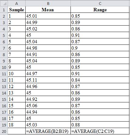
Date set:1
Table 4
| Sample | Mean | Range |
| 1 | 45.01 | 0.85 |
| 2 | 44.99 | 0.89 |
| 3 | 45.02 | 0.86 |
| 4 | 45 | 0.91 |
| 5 | 45.04 | 0.87 |
| 6 | 44.98 | 0.9 |
| 7 | 44.91 | 0.86 |
| 8 | 45.04 | 0.89 |
| 9 | 45 | 0.85 |
| 10 | 44.97 | 0.91 |
| 11 | 45.11 | 0.84 |
| 12 | 44.96 | 0.87 |
| 13 | 45 | 0.86 |
| 14 | 44.92 | 0.89 |
| 15 | 45.06 | 0.87 |
| 16 | 44.94 | 0.86 |
| 17 | 45 | 0.85 |
| 18 | 45.03 | 0.88 |
| 45 | 0.872777778 |
Excel worksheet:
From factors of three-sigma chart, for n=20, A2 = 0.18; D3 = 0.41; D4 = 1.59
Mean control chart:
Range control chart:
Upper control limit:
The upper control limit is calculated by adding the product of 0.18 and 0.873 with 45, which yields 45.156.
Lower control limit:
The lower control limit is calculated by subtracting the product of 0.18 and 0.873 with 45, which yields 44.842.
A graph is plotted using the UCL, LCL and samples values.
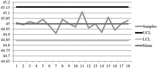
Diagram 1
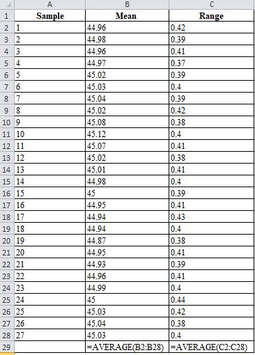
Date set: 2
Table 5
| Sample | Mean | Range |
| 1 | 44.96 | 0.42 |
| 2 | 44.98 | 0.39 |
| 3 | 44.96 | 0.41 |
| 4 | 44.97 | 0.37 |
| 5 | 45.02 | 0.39 |
| 6 | 45.03 | 0.4 |
| 7 | 45.04 | 0.39 |
| 8 | 45.02 | 0.42 |
| 9 | 45.08 | 0.38 |
| 10 | 45.12 | 0.4 |
| 11 | 45.07 | 0.41 |
| 12 | 45.02 | 0.38 |
| 13 | 45.01 | 0.41 |
| 14 | 44.98 | 0.4 |
| 15 | 45 | 0.39 |
| 16 | 44.95 | 0.41 |
| 17 | 44.94 | 0.43 |
| 18 | 44.94 | 0.4 |
| 19 | 44.87 | 0.38 |
| 20 | 44.95 | 0.41 |
| 21 | 44.93 | 0.39 |
| 22 | 44.96 | 0.41 |
| 23 | 44.99 | 0.4 |
| 24 | 45 | 0.44 |
| 25 | 45.03 | 0.42 |
| 26 | 45.04 | 0.38 |
| 27 | 45.03 | 0.4 |
| 44.9959 | 0.40111 |
Excel worksheet:
From factors of three-sigma chart, for n=20, A2 = 0.58
Mean control chart:
Range control chart:
Upper control limit:
The upper control limit is calculated by adding the product of 0.58 and 0.401 with 44.99, which yields 45.229.
Lower control limit:
The lower control limit is calculated by subtracting the product of 0.58 and 0.401 with 44.99, which yields 44.763.
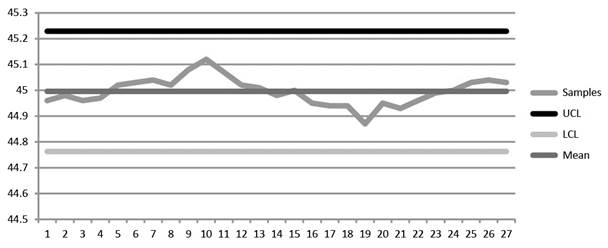
Diagram 2
On comparing Diagrams 1 and 2, it is evident that the second set of data has closer range of changes while the first set of data is scattered and reveals no information about the changes in the process.
Hence, the second sample reveals the changes in the process changes more clearly than the first set of data.
Want to see more full solutions like this?
Chapter 10 Solutions
EBK OPERATIONS MANAGEMENT


- Sarah Anderson, the Marketing Manager at Exeter Township's Cultural Center, is conducting research on the attendance history for cultural events in the area over the past ten years. The following data has been collected on the number of attendees who registered for events at the cultural center. Year Number of Attendees 1 700 2 248 3 633 4 458 5 1410 6 1588 7 1629 8 1301 9 1455 10 1989 You have been hired as a consultant to assist in implementing a forecasting system that utilizes various forecasting techniques to predict attendance for Year 11. a) Calculate the Three-Period Simple Moving Average b) Calculate the Three-Period Weighted Moving Average (weights: 50%, 30%, and 20%; use 50% for the most recent period, 30% for the next most recent, and 20% for the oldest) c) Apply Exponential Smoothing with the smoothing constant alpha = 0.2. d) Perform a Simple Linear Regression analysis and provide the adjusted…arrow_forwardRuby-Star Incorporated is considering two different vendors for one of its top-selling products which has an average weekly demand of 70 units and is valued at $90 per unit. Inbound shipments from vendor 1 will average 390 units with an average lead time (including ordering delays and transit time) of 4 weeks. Inbound shipments from vendor 2 will average 490 units with an average lead time of 2 weeksweeks. Ruby-Star operates 52 weeks per year; it carries a 4-week supply of inventory as safety stock and no anticipation inventory. Part 2 a. The average aggregate inventory value of the product if Ruby-Star used vendor 1 exclusively is $enter your response here.arrow_forwardSam's Pet Hotel operates 50 weeks per year, 6 days per week, and uses a continuous review inventory system. It purchases kitty litter for $13.00 per bag. The following information is available about these bags: > Demand 75 bags/week > Order cost = $52.00/order > Annual holding cost = 20 percent of cost > Desired cycle-service level = 80 percent >Lead time = 5 weeks (30 working days) > Standard deviation of weekly demand = 15 bags > Current on-hand inventory is 320 bags, with no open orders or backorders. a. Suppose that the weekly demand forecast of 75 bags is incorrect and actual demand averages only 50 bags per week. How much higher will total costs be, owing to the distorted EOQ caused by this forecast error? The costs will be $higher owing to the error in EOQ. (Enter your response rounded to two decimal places.)arrow_forward
- Yellow Press, Inc., buys paper in 1,500-pound rolls for printing. Annual demand is 2,250 rolls. The cost per roll is $625, and the annual holding cost is 20 percent of the cost. Each order costs $75. a. How many rolls should Yellow Press order at a time? Yellow Press should order rolls at a time. (Enter your response rounded to the nearest whole number.)arrow_forwardPlease help with only the one I circled! I solved the others :)arrow_forwardOsprey Sports stocks everything that a musky fisherman could want in the Great North Woods. A particular musky lure has been very popular with local fishermen as well as those who buy lures on the Internet from Osprey Sports. The cost to place orders with the supplier is $40/order; the demand averages 3 lures per day, with a standard deviation of 1 lure; and the inventory holding cost is $1.00/lure/year. The lead time form the supplier is 10 days, with a standard deviation of 2 days. It is important to maintain a 97 percent cycle-service level to properly balance service with inventory holding costs. Osprey Sports is open 350 days a year to allow the owners the opportunity to fish for muskies during the prime season. The owners want to use a continuous review inventory system for this item. Refer to the standard normal table for z-values. a. What order quantity should be used? lures. (Enter your response rounded to the nearest whole number.)arrow_forward
- In a P system, the lead time for a box of weed-killer is two weeks and the review period is one week. Demand during the protection interval averages 262 boxes, with a standard deviation of demand during the protection interval of 40 boxes. a. What is the cycle-service level when the target inventory is set at 350 boxes? Refer to the standard normal table as needed. The cycle-service level is ☐ %. (Enter your response rounded to two decimal places.)arrow_forwardOakwood Hospital is considering using ABC analysis to classify laboratory SKUs into three categories: those that will be delivered daily from their supplier (Class A items), those that will be controlled using a continuous review system (B items), and those that will be held in a two bin system (C items). The following table shows the annual dollar usage for a sample of eight SKUs. Fill in the blanks for annual dollar usage below. (Enter your responses rounded to the mearest whole number.) Annual SKU Unit Value Demand (units) Dollar Usage 1 $1.50 200 2 $0.02 120,000 $ 3 $1.00 40,000 $ 4 $0.02 1,200 5 $4.50 700 6 $0.20 60,000 7 $0.90 350 8 $0.45 80arrow_forwardA part is produced in lots of 1,000 units. It is assembled from 2 components worth $30 total. The value added in production (for labor and variable overhead) is $30 per unit, bringing total costs per completed unit to $60 The average lead time for the part is 7 weeks and annual demand is 3800 units, based on 50 business weeks per year. Part 2 a. How many units of the part are held, on average, in cycle inventory? enter your response here unitsarrow_forward
- assume the initial inventory has no holding cost in the first period and back orders are not permitted. Allocating production capacity to meet demand at a minimum cost using the transportation method. What is the total cost? ENTER your response is a whole number (answer is not $17,000. That was INCORRECT)arrow_forwardRegular Period Time Overtime Supply Available puewag Subcontract Forecast 40 15 15 40 2 35 40 28 15 15 20 15 22 65 60 Initial inventory Regular-time cost per unit Overtime cost per unit Subcontract cost per unit 20 units $100 $150 $200 Carrying cost per unit per month 84arrow_forwardassume that the initial inventory has no holding cost in the first period, and back orders are not permitted. Allocating production capacity to meet demand at a minimum cost using the transportation method. The total cost is? (enter as whole number)arrow_forward
 Practical Management ScienceOperations ManagementISBN:9781337406659Author:WINSTON, Wayne L.Publisher:Cengage,
 Foundations of Business (MindTap Course List)MarketingISBN:9781337386920Author:William M. Pride, Robert J. Hughes, Jack R. KapoorPublisher:Cengage Learning
 Foundations of Business - Standalone book (MindTa...MarketingISBN:9781285193946Author:William M. Pride, Robert J. Hughes, Jack R. KapoorPublisher:Cengage Learning