
Concept explainers
Videos
Heinz, a manufacturer of ketchup, uses a particular machine to dispense 16 ounces of its ketchup into containers. From many years of experience with the particular dispensing machine, Heinz knows the amount of product in each container follows a
- (a) State the null hypothesis and the alternate hypothesis.
- (b) What is the
probability of a Type I error? - (c) Give the formula for the test statistic.
- (d) State the decision rule.
- (e) Determine the value of the test statistic.
- (f) What is your decision regarding the null hypothesis?
- (g) Interpret, in a single sentence, the result of the statistical test.
a.
State the hypotheses.
Answer to Problem 1SR
The null hypothesis is
The alternative hypothesis is
Explanation of Solution
Here, the claim is that there is evidence that the mean amount dispensed is different from 16 ounces. This defines the alternative hypothesis.
Let
The hypotheses are given below:
Null hypothesis:
Alternative hypothesis:
b.
Write the probability of a Type I error
Explanation of Solution
Type I error:
Probability of rejecting
Here, the null hypothesis is rejected. But in actual the mean amount dispensed is 16 ounces.
c.
Write the formula for the test statistic.
Explanation of Solution
The formula for the test statistic is given below:
Where,
d.
Write the decision rule.
Explanation of Solution
Step-by-step procedure to obtain the critical value using MINITAB:
- Choose Graph > Probability Distribution Plot choose View Probability > OK.
- From Distribution, choose ‘Normal’ distribution.
- Click the Shaded Area tab.
- Choose Probability and Both Tail for the region of the curve to shade.
- Enter the Probability value as 0.05.
- Click OK.
Output using the MINITAB software is given below:
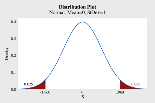
From the output, the critical value is ±1.96.
Decision rule:
If
If
e.
Find the value of test statistic.
Answer to Problem 1SR
The value of test statistic is 0.8.
Explanation of Solution
Step by step procedure to obtain the test statistic using MINITAB software is given below:
- Choose Stat > Basic Statistics > 1-Sample Z.
- In Summarized data, enter the sample size as 50 and mean as 16.017.
- In Standard deviation, enter 0.15.
- Check Options, enter Confidence level as 95.
- In Perform Hypothesis test, enter 16 Under Hypothesized mean.
- Choose Mean ≠ Hypothesized mean in alternative.
- Click OK in all dialogue boxes.
Output using the MINITAB software is given below:
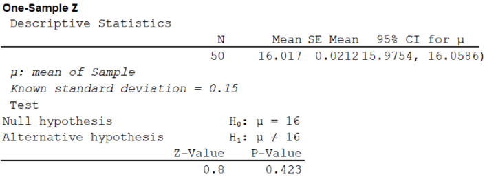
From the MINITAB output, the value of test statistic is 0.8.
f.
Find the decision.
Answer to Problem 1SR
The decision is that fail to reject the null hypothesis.
Explanation of Solution
Decision:
Here, the computed z-value is 0.8.
The computed z-value lies between ±1.96.
From the decision rule, fail to reject the null hypothesis.
g.
Write the single sentence for the result of the test.
Explanation of Solution
The null hypothesis is not rejected. Hence, it can be concluded that there is no evidence that the mean amount dispensed is different from 16 ounces.
Want to see more full solutions like this?
Chapter 10 Solutions
STAT. TECH. FOR BUSINESS AND ECO (LL)


- Suppose a random sample of 459 married couples found that 307 had two or more personality preferences in common. In another random sample of 471 married couples, it was found that only 31 had no preferences in common. Let p1 be the population proportion of all married couples who have two or more personality preferences in common. Let p2 be the population proportion of all married couples who have no personality preferences in common. Find a95% confidence interval for . Round your answer to three decimal places.arrow_forwardA history teacher interviewed a random sample of 80 students about their preferences in learning activities outside of school and whether they are considering watching a historical movie at the cinema. 69 answered that they would like to go to the cinema. Let p represent the proportion of students who want to watch a historical movie. Determine the maximal margin of error. Use α = 0.05. Round your answer to three decimal places. arrow_forwardA random sample of medical files is used to estimate the proportion p of all people who have blood type B. If you have no preliminary estimate for p, how many medical files should you include in a random sample in order to be 99% sure that the point estimate will be within a distance of 0.07 from p? Round your answer to the next higher whole number.arrow_forward
- A clinical study is designed to assess the average length of hospital stay of patients who underwent surgery. A preliminary study of a random sample of 70 surgery patients’ records showed that the standard deviation of the lengths of stay of all surgery patients is 7.5 days. How large should a sample to estimate the desired mean to within 1 day at 95% confidence? Round your answer to the whole number.arrow_forwardA clinical study is designed to assess the average length of hospital stay of patients who underwent surgery. A preliminary study of a random sample of 70 surgery patients’ records showed that the standard deviation of the lengths of stay of all surgery patients is 7.5 days. How large should a sample to estimate the desired mean to within 1 day at 95% confidence? Round your answer to the whole number.arrow_forwardIn the experiment a sample of subjects is drawn of people who have an elbow surgery. Each of the people included in the sample was interviewed about their health status and measurements were taken before and after surgery. Are the measurements before and after the operation independent or dependent samples?arrow_forward
- iid 1. The CLT provides an approximate sampling distribution for the arithmetic average Ỹ of a random sample Y₁, . . ., Yn f(y). The parameters of the approximate sampling distribution depend on the mean and variance of the underlying random variables (i.e., the population mean and variance). The approximation can be written to emphasize this, using the expec- tation and variance of one of the random variables in the sample instead of the parameters μ, 02: YNEY, · (1 (EY,, varyi n For the following population distributions f, write the approximate distribution of the sample mean. (a) Exponential with rate ẞ: f(y) = ß exp{−ßy} 1 (b) Chi-square with degrees of freedom: f(y) = ( 4 ) 2 y = exp { — ½/ } г( (c) Poisson with rate λ: P(Y = y) = exp(-\} > y! y²arrow_forward2. Let Y₁,……., Y be a random sample with common mean μ and common variance σ². Use the CLT to write an expression approximating the CDF P(Ỹ ≤ x) in terms of µ, σ² and n, and the standard normal CDF Fz(·).arrow_forwardmatharrow_forward
- Compute the median of the following data. 32, 41, 36, 42, 29, 30, 40, 22, 25, 37arrow_forwardTask Description: Read the following case study and answer the questions that follow. Ella is a 9-year-old third-grade student in an inclusive classroom. She has been diagnosed with Emotional and Behavioural Disorder (EBD). She has been struggling academically and socially due to challenges related to self-regulation, impulsivity, and emotional outbursts. Ella's behaviour includes frequent tantrums, defiance toward authority figures, and difficulty forming positive relationships with peers. Despite her challenges, Ella shows an interest in art and creative activities and demonstrates strong verbal skills when calm. Describe 2 strategies that could be implemented that could help Ella regulate her emotions in class (4 marks) Explain 2 strategies that could improve Ella’s social skills (4 marks) Identify 2 accommodations that could be implemented to support Ella academic progress and provide a rationale for your recommendation.(6 marks) Provide a detailed explanation of 2 ways…arrow_forwardQuestion 2: When John started his first job, his first end-of-year salary was $82,500. In the following years, he received salary raises as shown in the following table. Fill the Table: Fill the following table showing his end-of-year salary for each year. I have already provided the end-of-year salaries for the first three years. Calculate the end-of-year salaries for the remaining years using Excel. (If you Excel answer for the top 3 cells is not the same as the one in the following table, your formula / approach is incorrect) (2 points) Geometric Mean of Salary Raises: Calculate the geometric mean of the salary raises using the percentage figures provided in the second column named “% Raise”. (The geometric mean for this calculation should be nearly identical to the arithmetic mean. If your answer deviates significantly from the mean, it's likely incorrect. 2 points) Starting salary % Raise Raise Salary after raise 75000 10% 7500 82500 82500 4% 3300…arrow_forward
 Glencoe Algebra 1, Student Edition, 9780079039897...AlgebraISBN:9780079039897Author:CarterPublisher:McGraw Hill
 Big Ideas Math A Bridge To Success Algebra 1: Stu...AlgebraISBN:9781680331141Author:HOUGHTON MIFFLIN HARCOURTPublisher:Houghton Mifflin Harcourt