View the attatchments and then explain the following - Find the skewness and kurtosis of commuting times and explain what the box and whisker plot and data is showing or explaining.
View the attatchments and then explain the following - Find the skewness and kurtosis of commuting times and explain what the box and whisker plot and data is showing or explaining.

MATLAB: An Introduction with Applications
6th Edition
ISBN:9781119256830
Author:Amos Gilat
Publisher:Amos Gilat
Chapter1: Starting With Matlab
Section: Chapter Questions
Problem 1P

Related questions
Question
View the attatchments and then explain the following
- Find the skewness and kurtosis of commuting times and explain what the box and whisker plot and data is showing or explaining.

Transcribed Image Text:**Commuting Times (in minutes) Data Analysis**
The dataset consists of commuting times measured in minutes. Here are some key statistical measures derived from the data:
- **Minimum**: 10 minutes
- **First Quartile (Q1)**: 40 minutes
- **Median**: 60 minutes
- **Third Quartile (Q3)**: 120 minutes
- **Maximum**: 260 minutes
- **Mean**: 73.74 minutes
**Box Plot Explanation:**
The accompanying box plot provides a visual representation of the distribution of commuting times:
- **Box**: The central box represents the interquartile range (IQR), which contains the middle 50% of the data (from Q1 to Q3). For this dataset, it ranges from 40 to 120 minutes.
- **Median Line**: Inside the box, a line indicates the median at 60 minutes, showcasing where the center of the data lies.
- **Whiskers**: The whiskers extend to the smallest and largest values within 1.5 times the IQR from Q1 and Q3, respectively. The lower whisker bottoms at 10 minutes.
- **Outliers**: Any data points beyond the whiskers are considered outliers. In this plot, the dot above the upper whisker at 260 minutes represents an outlier, indicating a significantly longer commuting time compared to most of the data.
This box plot is a helpful tool for quickly visualizing the distribution, central tendency, and variability of commuting times in the dataset, as well as identifying any potential outliers.

Transcribed Image Text:**Commuting Times (in minutes)**
20
45
90
15
40
150
120
40
60
80
80
60
30
90
60
30
30
260
120
120
30
30
90
10
120
120
45
60
12
80
50
40
120
50
30
40
60
45
120
50
40
40
120
120
200
10
65
40
60
60
120
140
Expert Solution
Step 1
Given data of commuting times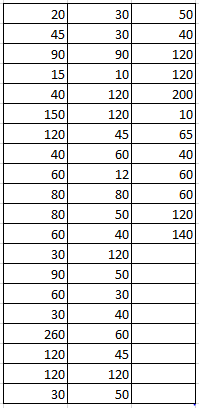
Using this data we can use excel functions =Skew() to find skewness and =KURT() to find kurtosis

Step by step
Solved in 2 steps with 2 images

Recommended textbooks for you
MATLAB: An Introduction with Applications
Statistics
ISBN:
9781119256830
Author:
Amos Gilat
Publisher:
John Wiley & Sons Inc

Probability and Statistics for Engineering and th…
Statistics
ISBN:
9781305251809
Author:
Jay L. Devore
Publisher:
Cengage Learning

Statistics for The Behavioral Sciences (MindTap C…
Statistics
ISBN:
9781305504912
Author:
Frederick J Gravetter, Larry B. Wallnau
Publisher:
Cengage Learning
MATLAB: An Introduction with Applications
Statistics
ISBN:
9781119256830
Author:
Amos Gilat
Publisher:
John Wiley & Sons Inc
Probability and Statistics for Engineering and th…
Statistics
ISBN:
9781305251809
Author:
Jay L. Devore
Publisher:
Cengage Learning
Statistics for The Behavioral Sciences (MindTap C…
Statistics
ISBN:
9781305504912
Author:
Frederick J Gravetter, Larry B. Wallnau
Publisher:
Cengage Learning

Elementary Statistics: Picturing the World (7th E…
Statistics
ISBN:
9780134683416
Author:
Ron Larson, Betsy Farber
Publisher:
PEARSON

The Basic Practice of Statistics
Statistics
ISBN:
9781319042578
Author:
David S. Moore, William I. Notz, Michael A. Fligner
Publisher:
W. H. Freeman

Introduction to the Practice of Statistics
Statistics
ISBN:
9781319013387
Author:
David S. Moore, George P. McCabe, Bruce A. Craig
Publisher:
W. H. Freeman