
Concept explainers
Speed and density The following data relate traffic Density (measured as number of cars per mile) and the average Speed of traffic (in mph) on city highways. The data were collected at the same location at 10 different times randomly selected within a span of 3 months.
| Density | Speed | |
| 69 | 25.4 | |
| 56 | 32.5 | |
| 62 | 28.6 | |
| 119 | 11.5 | |
| 84 | 21.3 | |
| 74 | 22.1 | |
| 73 | 22.3 | |
| 90 | 18.5 | |
| 38 | 37.2 | |
| 22 | 44.6 | |
| Mean | 68.7 | 26.4 |
| SD | 27.07 | 9.64 |
- a) Describe the relationship between Speed and Density.
- b) Fit a model to predict Speed from Density. Comment on the appropriateness of the model.
- c) If the traffic density is 56 cars/mile and you observe a speed of 32.5 mph, what is the residual? What is the residual for an observed speed of 36.1 mph with a traffic density of 20 cars/mile?
- d) Which of the two residuals in part c is more unusual? Explain.
- e) A new data point has come in. For this observation, Density = 125 cars/mile and Speed = 55 mph. What would happen to the slope and the
correlation if this point were included? - f) Predict the speed of traffic for a density of 200 cars/mile. Is your prediction reasonable? Explain briefly.
- g) If you standardize both variables, what equation predicts the standardized speed from the standardized density?
- h) If you standardize both variables, what equation predicts the standardized density from the standardized speed?
a.
Explain the relationship between speed and density.
Explanation of Solution
Given info:
The data related to the speed and density of traffic at the same location of a city at 10 different times within a span of 3 months.
Calculation:
Scatterplot:
Software procedure:
Step by step procedure to draw scatterplot using MINITAB software is given as,
- Choose Graph > Scatterplot.
- Choose Simple, and then click OK.
- In Y-variables, enter the column of Speed.
- In X-variables enter the column of Density.
- Click OK.
Output using MINITAB software is given as,
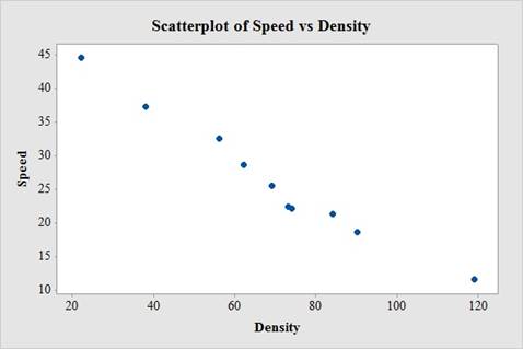
The relation between speed and density is strong, negative and linear. Thus, the association between speed and density is associated with lower speeds.
b.
Obtain a linear model to predict speed from density and comment on the appropriateness of the model.
Answer to Problem 4E
The regression equation of linear model is
Explanation of Solution
Calculation:
Linear regression model:
A linear regression model is given as
Regression
Software procedure:
Step by step procedure to get the output using MINITAB software is given as,
- Choose Stat > Regression > Regression > Fit Regression Model.
- Under Responses, enter the column of Speed.
- Under predictors, enter the columns of Density.
- Click OK.
Output using MINITAB software is given below:
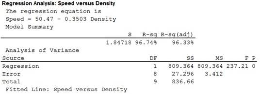
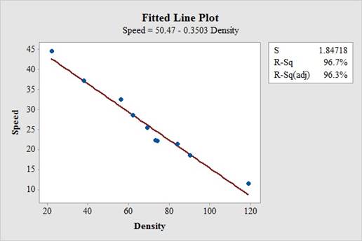
Thus, the regression equation of linear model is
The fitted scatterplot of re-expressed data exhibits a linear pattern. Thus, there is a strong and negative linear association between speed and density of traffic
The coefficient of determination (
In the given output,
Thus, the percentage of variation in the observed values of speed of traffic that is explained by the regression is 96.7%, which indicates that 96.7% of the variability in speed is explained by the variability in density using linear regression model.
The conditions for a residual plot that is well fitted for the data are,
- There should not any bend, which would violate the straight enough condition.
- There must not any outlier, which, were not clear before.
- There should not any change in the spread of the residuals from one part to another part of the plot.
Residual plot:
Software procedure:
Step by step procedure to get the output using MINITAB software is given as,
- Choose Stat > Regression > Regression > Fit Regression Model.
- Under Responses, enter the column of Speed.
- Under Continuous predictors, enter the columns of Density.
- In Graphs, under Residuals for plots choose Regular.
- Under Residuals plots choose Individuals plots and select box of Residuals versus fits.
- Click OK.
Output using MINITAB software is given below:
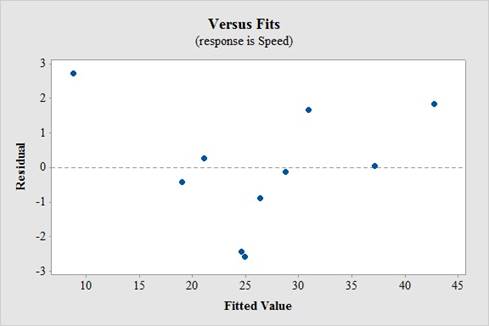
In residual plot, there is no bend or pattern, which can violate the straight enough condition and there is no change in the spread of the residuals from one part to another part of the plot.
Thus, a linear model is appropriated.
c.
Find the residual of a traffic, having density and observed speed of 56 cars/mile and 32.5 mph, respectively.
Find the residual of another traffic, having density and observed speed of 20 cars/mile and 36.1 mph, respectively.
Answer to Problem 4E
The residual of a traffic, having density and observed speed of 56 cars/mile and 32.5 mph, respectively is 1.65 mph and the residual of a traffic, having density and observed speed of 20 cars/mile and 36.1 mph, respectively is –7.36 mph.
Explanation of Solution
Calculation:
Assume x be the predictor variable and y be the response variable, of a regression analysis. Then, the predicted value of the response variable is
Residual:
The residual is defined as
If the observed value is less than predicted value then the residual will be negative and if the observed value is greater than predicted value then the residual will be positive.
From the previous part b. it is found that the regression equation of linear model is
The predicted speed of a traffic having density of 56 cars/mile is,
Thus, the predicted speed of a traffic having density of 56 cars/mile is 30.8532 mph.
It is known, that actual speed of a traffic having density of 56 cars/mile is 32.5 mph.
The value of the residual is,
Thus, the residual of a traffic, having density and observed speed of 56 cars/mile and 32.5 mph, respectively is 1.65 mph.
The predicted speed of a traffic having density of 20 cars/mile is,
Thus, the predicted speed of a traffic having density of 20 cars/mile is 43.46 mph.
It is known, that actual speed of a traffic having density of 20 cars/mile is 36.1 mph.
The value of the residual is,
Thus, the residual of a traffic, having density and observed speed of 20 cars/mile and 36.1 mph, respectively is –7.36 mph.
d.
Find the unusual residual.
Answer to Problem 4E
Second residual is more unusual residual.
Explanation of Solution
From previous part c. it is found that residual of a traffic, having density and observed speed of 56 cars/mile and 32.5 mph, respectively is 1.65 mph and the residual of a traffic, having density and observed speed of 20 cars/mile and 36.1 mph, respectively is –7.36 mph.
Thus, it is clear that the second residual value is far away from the predicted value. Therefore, second residual is more unusual residual.
e.
Explain about slope and the correlation if the new point
Explanation of Solution
The new point
In another words, shallower slope and weaker correlation are closer to 0 as they are both started as negative quantity.
Thus, technically slope and correlation becomes higher.
f.
Predict the speed of traffic for a density of 200 cars/mile.
Explain whether the prediction is reasonable.
Answer to Problem 4E
The predicted speed of a traffic having density of 200 cars/mile is –19.6 mph.
Explanation of Solution
Calculation:
The predicted speed of a traffic having density of 200 cars/mile is,
Thus, the predicted speed of a traffic having density of 200 cars/mile is –19.6 mph.
This result is not meaningful as the value of the speed comes as negative quantity, which cannot be possible. Moreover, the given car density of 200 cars/mile is far beyond from the observed values.
Thus, the prediction is not reasonable.
g.
Find the equation to predict the standardized speed from the standardized density if both the variables are standardized.
Answer to Problem 4E
The equation to predict the standardized speed from the standardized density is
Explanation of Solution
Calculation:
z-score:
The z-score of a random variable x is defined as
Correlation coefficient:
Software Procedure:
Step by step procedure to obtain the correlation coefficient of the data using the MINITAB software:
- Choose Stat > Basic Statistics > Correlation.
- In Variables, enter the column of Speed and Density.
- Click OK in all dialogue boxes.
Output using the MINITAB software is given below:

Thus, the correlation confident for speed and density is –0.984.
It is known that, the slope
Now, for the predictor variable x and response variable y also scarify the regression equation
Consider, the mean of the predictor variable x is
Subtract the equation
Using the formula
In this problem, as speed is the predictor variable (x) and density of traffic is response variable (y) with the correlation coefficient of
h.
Find the equation to predict the standardized density from the standardized speed if both the variables are standardized.
Answer to Problem 4E
The equation to predict the standardized density from the standardized speed is
Explanation of Solution
Calculation:
From the previous part g. it is found that the correlation confident for speed and density is –0.984. In addition correlation is same regardless of the direction of prediction.
Consider, the mean of the predictor variable x is
Subtract the equation
Using the formula
In this problem, as density is the predictor variable (x) and speed of traffic is response variable (y) with the correlation coefficient of
Want to see more full solutions like this?
Chapter CR Solutions
Intro Stats, Books a la carte Plus NEW MyLab Statistics with Pearson eText -- Access Card Package (5th Edition)
- A college wants to estimate what students typically spend on textbooks. A report fromthe college bookstore observes that textbooks range in price from $22 to $186. Toobtain a 95% confidence level for a confidence interval estimate to plus or minus $10,how many students should the college survey? (We may estimate the populationstandard deviation as (range) ÷ 4.)arrow_forwardIn a study of how students give directions, forty volunteers were given the task ofexplaining to another person how to reach a destination. Researchers measured thefollowing five aspects of the subjects’ direction-giving behavior:• whether a map was available or if directions were given from memory without a map,• the gender of the direction-giver,• the distances given as part of the directions,• the number of times directions such as “north” or “left” were used,• the frequency of errors in directions. Identify each of the variables in this study, and whether each is quantitative orqualitative. For each quantitative variable, state whether it is discrete or continuous. Was this an observational study or an experimental study? Explain your answer.arrow_forwardexplain the difference between the confident interval and the confident level. provide an example to show how to correctly interpret a confidence interval.arrow_forward
- Sketch to scale the orbit of Earth about the sun. Graph Icarus’ orbit on the same set of axesWhile the sun is the center of Earth’s orbit, it is a focus of Icarus’ orbit. There aretwo points of intersection on the graph. Based on the graph, what is the approximate distance between the two points of intersection (in AU)?arrow_forwardThe diameters of ball bearings are distributed normally. The mean diameter is 67 millimeters and the standard deviation is 3 millimeters. Find the probability that the diameter of a selected bearing is greater than 63 millimeters. Round to four decimal places.arrow_forwardSuppose you like to keep a jar of change on your desk. Currently, the jar contains the following: 22 Pennies 27 Dimes 9 Nickels 30 Quarters What is the probability that you reach into the jar and randomly grab a penny and then, without replacement, a dime? Express as a fraction or a decimal number rounded to four decimal places.arrow_forward
- A box contains 14 large marbles and 10 small marbles. Each marble is either green or white. 9 of the large marbles are green, and 4 of the small marbles are white. If a marble is randomly selected from the box, what is the probability that it is small or white? Express as a fraction or a decimal number rounded to four decimal places.arrow_forwardCan I get help with this step please? At a shooting range, instructors can determine if a shooter is consistently missing the target because of the gun sight or because of the shooter's ability. If a gun's sight is off, the variance of the distances between the shots and the center of the shot pattern will be small (even if the shots are not in the center of the target). A student claims that it is the sight that is off, not his aim, and wants the instructor to confirm his claim. If a skilled shooter fires a gun at a target multiple times, the distances between the shots and the center of the shot pattern, measured in centimeters (cm), will have a variance of less than 0.33. After the student shoots 28 shots at the target, the instructor calculates that the distances between his shots and the center of the shot pattern, measured in cm, have a variance of 0.25. Does this evidence support the student's claim that the gun's sight is off? Use a 0.025 level of significance. Assume that the…arrow_forwardThe National Academy of Science reported that 38% of research in mathematics is published by US authors. The mathematics chairperson of a prestigious university wishes to test the claim that this percentage is no longer 38%. He has no indication of whether the percentage has increased or decreased since that time. He surveys a simple random sample of 279 recent articles published by reputable mathematics research journals and finds that 123 of these articles have US authors. Does this evidence support the mathematics chairperson's claim that the percentage is no longer 38 % ? Use a 0.02 level of significance. Compute the value of the test statistic. Round to two decimal places.arrow_forward
- A marketing research company desires to know the mean consumption of milk per week among males over age 32. They believe that the milk consumption has a mean of 4 liters, and want to construct a 98% confidence interval with a maximum error of 0.07 liters. Assuming a variance of 0.64 liters, what is the minimum number of males over age 32 they must include in their sample? Round up to the next integer.arrow_forwardSuppose GRE Verbal scores are normally distributed with a mean of 461 and a standard deviation of 118. A university plans to recruit students whose scores are in the top 4 % . What is the minimum score required for recruitment? Round to the nearest whole number, if necessaryarrow_forwardNeed help with my homework thank you random sample of 6 fields of durum wheat has a mean yield of 45.5 bushels per acre and standard deviation of 7.43 bushels per acre. Determine the 80 % confidence interval for the true mean yield. Assume the population is approximately normal. Step 1: Find the critical value that should be used in constructing the confidence interval. Round to three decimal places. Step 2 of 2: Construct the 80% confidence interval. Round to one decimal place. I got 1.476 as my critical value and 41.0 and 49.9 as my confidence intervalarrow_forward
 Holt Mcdougal Larson Pre-algebra: Student Edition...AlgebraISBN:9780547587776Author:HOLT MCDOUGALPublisher:HOLT MCDOUGAL
 Functions and Change: A Modeling Approach to Coll...AlgebraISBN:9781337111348Author:Bruce Crauder, Benny Evans, Alan NoellPublisher:Cengage Learning
 Glencoe Algebra 1, Student Edition, 9780079039897...AlgebraISBN:9780079039897Author:CarterPublisher:McGraw Hill
 Big Ideas Math A Bridge To Success Algebra 1: Stu...AlgebraISBN:9781680331141Author:HOUGHTON MIFFLIN HARCOURTPublisher:Houghton Mifflin Harcourt


