Chapter 9.3, Problem 2CYU

a.

To determine

State the null and alternate hypotheses.

Answer to Problem 2CYU

The hypotheses are given below:

Null hypothesis:

$H_0:{\mu }_d=0$

That is, there is no significant difference between the mean amount of rainfall of a city in year2 and year1.

Alternate hypothesis:

$H_1:{\mu }_d>0$

That is, the mean amount of rainfall of the city in year2 is greater than the mean amount of rainfall of the city in year1.

Explanation of Solution

The data represents the mean amount of rainfall of a chosen city in two consecutive years (year2 and year1).

Hypothesis:

Hypothesis is an assumption about the parameter of the population, and the assumption may or may not be true.

Let ${\mu }_d$ be the population mean difference in rainfall of a city in year2 and year1 (Year2 – Year1).

Claim:

Here, the claim is, whether the mean amount of rainfall of the city in year2 is greater than the mean amount of rainfall of the city in year1.

The hypotheses are given below:

Null hypothesis:

Null hypothesis is a statement which is tested for statistical significance in the test. The decision criterion indicates whether the null hypothesis will be rejected or not in the favor of alternate hypothesis.

$H_0:{\mu }_d=0$

That is, there is no significant difference between the mean amount of rainfall of a city in year2 and year1.

Alternate hypothesis:

Alternate hypothesis is contradictory statement of the null hypothesis

$H_1:{\mu }_d>0$

That is, the mean amount of rainfall of the city in year2 is greater than the mean amount of rainfall of the city in year1.

b.

To determine

Compute the differences in amount of rainfalls Year2– Year1.

Answer to Problem 2CYU

The differences in amount of rainfalls Year2– Year1 is,

S.no	$\text{Difference}$
1	9.5
2	3.4
3	–3.8
4	10.1
5	8.9
6	5.7

Explanation of Solution

Calculation:

The differences in amount of rainfalls Year2– Year1 is,

S.no	Year2	Year1	$\text{Difference}\text{=}\text{After}-\text{Before}$
1	34.6	25.1	$34.6-25.1=9.5$
2	18.7	15.3	$18.7-15.3=3.4$
3	42.6	46.4	$42.6-46.4=-3.8$
4	41.3	31.2	$41.3-31.2=10.1$
5	60.6	51.7	$60.6-51.7=8.9$
6	29.9	24.2	$29.9-24.2=5.7$

c.

To determine

Find the value of t-test statistic.

Answer to Problem 2CYU

The value of test statistic is 2.6118.

Explanation of Solution

Calculation:

Test statistic:

The test statistic for matched pairs is obtained as,

$t=\frac{\overline{d}-{\mu }_0}{\left(\frac{s_d}{\sqrt{n}}\right)}$,

where $\overline{d}$ is the sample mean of the differences between the values in the matched pairs, $s_d$ is the sample standard deviation of the differences between the values in the

matched pairs and ${\mu }_d$ is the population mean difference for matched pair.

Mean and standard deviation of differences:

Software procedure:

Step-by-step procedure to obtain the mean and standard deviation using the MINITAB software:

• Choose Stat > Basic statistic > Display descriptive statistics.
• In Variables, enter the column of Differences.
• In Statistics, select mean, standard deviation and N total.
• Click OK.

Output using the MINITAB software is given below:

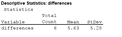
From the MINITAB output, the mean and standard deviation are 5.63 and 5.28.

The mean and standard deviation of the differences is 5.63 and 5.28.

Here, the sample size is $n=6$.

The test statistic is obtained as follows,

$\begin{array}{c}t=\frac{\overline{d}-0}{\left(\frac{s_d}{\sqrt{n}}\right)}\\ =\frac{5.63-0}{\left(\frac{5.28}{\sqrt{6}}\right)}\\ =\frac{5.63}{2.1556}\\ =2.6118\end{array}$

Thus, the test statistic is 2.6118.

d.

To determine

Find the P-value for the test statistic.

Answer to Problem 2CYU

The P-value for the test statistic is 0.02378.

Explanation of Solution

Calculation:

Degrees of freedom:

The degrees of freedom for the test statistic is,

$\begin{array}{c}d.f=n-1\\ =6-1\\ =5\end{array}$

Thus, the degree of freedom is 5.

P-value:

Software procedure:

Step-by-step procedure to obtain the P-value using the MINITAB software:

• Choose Graph > Probability Distribution Plot.
• Choose View Probability > OK.
• From Distribution, choose ‘t’ distribution.
• In Degrees of freedom, enter 5.
• Click the Shaded Area tab.
• Choose X value and Right Tail for the region of the curve to shade.
• In X-value enter 2.6118.
• Click OK.

Output using the MINITAB software is given below:

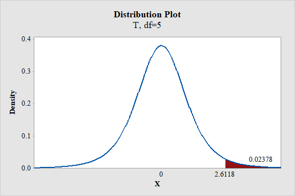
From the MINITAB output, the P-value is 0.02378.

Thus, the P-value is 0.02378.

e.

To determine

Interpret the P-value at the level of significance $\alpha =0.05$.

Answer to Problem 2CYU

There is enough evidence to reject the null hypothesis $H_0$.

Explanation of Solution

From part (d), the P-value is 0.02378.

Decision rule based on P-value:

If $P-\text{value}\le \alpha$, then reject the null hypothesis $H_0$.

If $P-\text{value}>\alpha$, then fail to reject the null hypothesis $H_0$.

Here, the level of significance is $\alpha =0.05$.

Conclusion based on P-value approach:

The P-value is 0.02378 and $\alpha$ value is 0.05.

Here, P-value is less than the $\alpha$ value.

That is, $0.02378\left(=P-\text{value}\right)<0.05\left(=\alpha \right)$.

By the rejection rule, reject the null hypothesis.

Thus, there is enough evidence to reject the null hypothesis $H_0$.

f.

To determine

State the conclusion.

Answer to Problem 2CYU

There is enough evidence to conclude that the mean amount of rainfall of the city in year2 is greater than the mean amount of rainfall of the city in year1.

Explanation of Solution

From part (e), it is known that the null hypothesis is rejected.

That is, mean amount of rainfall of the city in year2 is greater than the mean amount of rainfall of the city in year1.

Thus, there is enough evidence to conclude that the mean amount of rainfall of the city in year2 is greater than the mean amount of rainfall of the city in year1.