
Videos
In Problems 8-12, please use the following steps (i)-(v) for all hypothesis tests:
(i) What is the level of significance? State the null and alternate hypotheses.
(ii) Check Requirements What sampling distribution will you use? What assumptions are you making? What is the value of the sample test statistic?
(iii) Find (or estimate) the P-value. Sketch the sampling distribution and show the area corresponding to the P-value.
(iv) Based on your answers in parts (i)-(iii), will you reject or fail to reject the null hypothesis? Are the data statistically significant at level a?
(v) Interpret your conclusion in the context of the application.
Note: For degrees of freedom d.f. not in the Student’s t table, use the closet d.f. that is smaller. In some situation, this choice of d.f. may increase the P-value a small amount and thereby produce a slightly more "conservative” answer.
Testing and Estimating µ with σ Unknown Carboxyhemoglobin is formed when hemoglobin is exposed to carbon monoxide. Heavy smokers tend to have a high percentage of carboxyhemoglobin in their blood (Reference: A Manual of Laboratory and Diagnostic Tests by F. Fischbach). Let x be a random variable representing percentage of carboxyhemoglobin in the blood. For a person who is a regular heavy smoker, x has a distribution that is approximately normal. A random sample of n = 12 blood tests given to a heavy smoker gave the following results (percentage of carboxyhemoglobin in the blood):
| 9.1 | 9.5 | 10.2 | 9.8 | 11.3 | 12.2 |
| 11.6 | 10.3 | 8.9 | 9.7 | 13.4 | 9.9 |
(a) Use a calculator to verify that
(b) A long-term population
(c) Use the given data to find a 99% confidence interval for µ for this patient.
(a)
Whether the sample mean
Answer to Problem 9CRP
Solution:
Yes, the sample mean
Explanation of Solution
To calculate the required statistics using the Minitab, follow the below instructions:
Step 1: Go to the Minitab software.
Step 2: Go to Stat >Basic statistics > Display Descriptive Statistics.
Step 3: Select ‘Percentages’ in variables.
Step 4: Click on OK.
The obtained statistics is:
Descriptive Statistics: Percentages
Statistics
| Variable | N | N* | Mean | SE Mean | StDev | Minimum | Q1 | Median | Q3 | Maximum |
| Percentages | 12 | 0 | 10.492 | 0.392 | 1.358 | 8.900 | 9.550 | 10.050 | 11.525 | 13.400 |
From the Minitab output, the sample mean and sample standard deviation are approximately equals to
(b)
(i)
The level of significance, null and alternative hypothesis.
Answer to Problem 9CRP
Solution:
The level of significance is
Explanation of Solution
The level of significance is defined as the probability of rejecting the null hypothesis when it is true, it is denoted by
Null hypothesis
Alternative hypothesis
(ii)
To find:
The sampling distribution that should be used and compute the value of the sample test statistic.
Answer to Problem 9CRP
Solution:
The student's t distribution should be used. The sample test statisticis 1.25.
Explanation of Solution
Calculation:
We assume that x distribution is mound shape and symmetrical, because
Using
The sample test statistic t is
(iii)
To find:
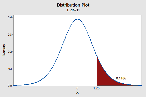
The P-value of the test statistic and sketch the sampling distribution showing the area corresponding to the P-value.
Answer to Problem 9CRP
Solution:
The P-value of the test statistic is 0.1186.
Explanation of Solution
Calculation:
We have t = 1.25
Using Table 4 from the Appendix to find the specified area:
Graph:
To draw the required graphs using the Minitab, follow the below instructions:
Step 1: Go to the Minitab software.
Step 2: Go to Graph > Probability distribution plot > View probability.
Step 3: Select ‘t’ and enter d.f = 11.
Step 4: Click on the Shaded area > X value.
Step 5: Enter X-value as 1.25 and select ‘Right Tail’.
Step 6: Click on OK.
The obtained distribution graph is:
(iv)
Whether we reject or fail to reject the null hypothesisand whether the data is statistically significant for a level of significance of 0.05.
Answer to Problem 9CRP
Solution:
The P-value
Explanation of Solution
The P-value of 0.1186 is greater than the level of significance (α) of 0.05. Therefore we failed to reject the null hypothesis
(v)
The interpretation for the conclusion.
Answer to Problem 9CRP
Solution:
There is not enough evidence to conclude that sample mean of 12 smokers' Carboxyhoemoglobin levels is significantly large enough to sound a clinical alert.
Explanation of Solution
The P-value is greater than the level of significance (
(b)
To find:
A 99% confidence interval for the mean for this patient.
Answer to Problem 9CRP
Solution:
The 99% confidence interval for
Explanation of Solution
Calculation:
We have to find 99% confidence interval
Then, the 99% confidence interval is
The 99% confidence interval for
Want to see more full solutions like this?
Chapter 9 Solutions
EBK UNDERSTANDING BASIC STATISTICS


- Name Harvard University California Institute of Technology Massachusetts Institute of Technology Stanford University Princeton University University of Cambridge University of Oxford University of California, Berkeley Imperial College London Yale University University of California, Los Angeles University of Chicago Johns Hopkins University Cornell University ETH Zurich University of Michigan University of Toronto Columbia University University of Pennsylvania Carnegie Mellon University University of Hong Kong University College London University of Washington Duke University Northwestern University University of Tokyo Georgia Institute of Technology Pohang University of Science and Technology University of California, Santa Barbara University of British Columbia University of North Carolina at Chapel Hill University of California, San Diego University of Illinois at Urbana-Champaign National University of Singapore…arrow_forwardA company found that the daily sales revenue of its flagship product follows a normal distribution with a mean of $4500 and a standard deviation of $450. The company defines a "high-sales day" that is, any day with sales exceeding $4800. please provide a step by step on how to get the answers in excel Q: What percentage of days can the company expect to have "high-sales days" or sales greater than $4800? Q: What is the sales revenue threshold for the bottom 10% of days? (please note that 10% refers to the probability/area under bell curve towards the lower tail of bell curve) Provide answers in the yellow cellsarrow_forwardFind the critical value for a left-tailed test using the F distribution with a 0.025, degrees of freedom in the numerator=12, and degrees of freedom in the denominator = 50. A portion of the table of critical values of the F-distribution is provided. Click the icon to view the partial table of critical values of the F-distribution. What is the critical value? (Round to two decimal places as needed.)arrow_forward
- A retail store manager claims that the average daily sales of the store are $1,500. You aim to test whether the actual average daily sales differ significantly from this claimed value. You can provide your answer by inserting a text box and the answer must include: Null hypothesis, Alternative hypothesis, Show answer (output table/summary table), and Conclusion based on the P value. Showing the calculation is a must. If calculation is missing,so please provide a step by step on the answers Numerical answers in the yellow cellsarrow_forwardShow all workarrow_forwardShow all workarrow_forward
 College Algebra (MindTap Course List)AlgebraISBN:9781305652231Author:R. David Gustafson, Jeff HughesPublisher:Cengage Learning
 Glencoe Algebra 1, Student Edition, 9780079039897...AlgebraISBN:9780079039897Author:CarterPublisher:McGraw Hill
 Holt Mcdougal Larson Pre-algebra: Student Edition...AlgebraISBN:9780547587776Author:HOLT MCDOUGALPublisher:HOLT MCDOUGAL