Chapter 9, Problem 9.28P

To determine

The expressions for the bandwidths of the circuits as shown in figures 1 and 2.

Answer to Problem 9.28P

The expressions for the bandwidths are:

For circuit in figure 1, $\left(0,\frac{1}{3}\sqrt{\frac{1}{R^2{C}^2}-1}\right)$

For circuit in figure 2,

$\left(0,\frac{1}{3}\sqrt{\left(\frac{2}{G}-1\right)\left(\frac{1}{R^2{C}^2}-1\right)}\right)$

Explanation of Solution

Given:

The circuits are as shown below:

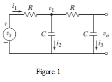
Concept Used:

1. Kirchhoff’s current and voltage laws are employed for finding the circuit equations.
2. The bandwidth of a system having transfer function as $T(\omega )=M\left(\omega \right)\angle \varphi \left(\omega \right)$, is:

$({\omega }_1,{\omega }_2)$ such that $M\left({\omega }_1\right)\le \frac{M_{peak}}{\sqrt{2}}\le M\left({\omega }_2\right)$.

Calculation:

For the circuit as shown in figure 1, on applying Kirchhoff’s voltage law:

$\begin{array}{l}{v}_1=i_{3}R+v_0\\ \Rightarrow i_3=\frac{v_1-v_0}{R}\end{array}$

And the current $i_3$ can be expressed as:

$i_3=C\frac{d{v}_0}{dt}$

Thus,

$\begin{array}{l}{i}_3=\frac{v_1-v_0}{R}\\ \Rightarrow C\frac{d{v}_0}{dt}=\frac{v_1-v_0}{R}\end{array}$

On taking Laplace transform of this, we get

$\begin{array}{l}C\frac{d{v}_0}{dt}=\frac{v_1-v_0}{R}\\ \Rightarrow RCs{V}_0\left(s\right)=V_1\left(s\right)-V_0\left(s\right)\\ \Rightarrow \frac{V_0\left(s\right)}{V_1\left(s\right)}=\frac{1}{\left(1+RCs\right)}\left(1\right)\end{array}$

Also, for the circuit in figure 1, on applying Kirchhoff’s current law:

$\begin{array}{l}{i}_1=i_2+i_3\\ \Rightarrow \frac{v_s-v_1}{R}=C\frac{d{v}_1}{dt}+C\frac{d{v}_0}{dt}\end{array}$

On taking the Laplace transform of this, we get

$\begin{array}{l}\frac{v_s-v_1}{R}=C\frac{d{v}_1}{dt}+C\frac{d{v}_0}{dt}\\ \Rightarrow V_s\left(s\right)-V_1\left(s\right)=sRC\left(V_1\left(s\right)+V_0\left(s\right)\right)\\ \Rightarrow V_s\left(s\right)-sRC{V}_0\left(s\right)=\left(sRC+1\right)V_1\left(s\right)\\ \Rightarrow V_1\left(s\right)=\left(\frac{V_s\left(s\right)-sRC{V}_0\left(s\right)}{\left(sRC+1\right)}\right)\left(2\right)\end{array}$

Thus, from equation (1) and (2), we have

$\begin{array}{l}{V}_0\left(s\right)=\frac{V_1\left(s\right)}{\left(1+RCs\right)}\\ \Rightarrow V_0\left(s\right)=\frac{V_s\left(s\right)-sRC{V}_0\left(s\right)}{{\left(sRC+1\right)}^2}\\ \Rightarrow V_0\left(s\right)\left({\left(sRC+1\right)}^2+sRC\right)=V_s\left(s\right)\\ \Rightarrow \frac{V_0\left(s\right)}{V_s\left(s\right)}=\frac{1}{R^2{C}^2{s}^2+3RCs+1}\end{array}$

This is the transfer function of the given circuit of figure 1.

Thus, the magnitude for this function is:

$M\left(\omega \right)=\frac{1}{\sqrt{{\left(1-R^2{C}^2\right)}^2+{\left(3RC\omega \right)}^2}}$

And the peak value for this magnitude occurs at $\omega =0$, that is

$M_{peak}=\frac{1}{\left(1-R^2{C}^2\right)}$

Thus, lower bound for the bandwidth is ${\omega }_1=0$ and the upper bound ${\omega }_2$ is:

$\begin{array}{l}M\left({\omega }_2\right)\ge \frac{M_{peak}}{\sqrt{2}}\\ \Rightarrow M^2\left({\omega }_2\right)\ge \frac{M_{peak}^2}{2}\\ \Rightarrow \frac{1}{{\left(1-R^2{C}^2\right)}^2+{\left(3RC{\omega }_2\right)}^2}\ge \frac{1}{2\left(1-R^2{C}^2\right)}\\ \Rightarrow {\left(1-R^2{C}^2\right)}^2+{\left(3RC{\omega }_2\right)}^2\le 2\left(1-R^2{C}^2\right)\\ \Rightarrow {\left(3RC{\omega }_2\right)}^2\le \left(1-R^2{C}^2\right)\\ \Rightarrow {\omega }_2\le \frac{1}{3}\sqrt{\frac{1}{R^2{C}^2}-1}\end{array}$

Therefore, the bandwidth of the circuit is:

$\left(0,\frac{1}{3}\sqrt{\frac{1}{R^2{C}^2}-1}\right)$

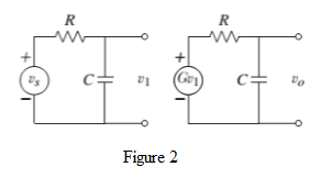
Similarly, for the circuit shown in figure 2, we have

$\frac{V_0\left(s\right)}{V_s\left(s\right)}=\frac{G}{R^2{C}^2{s}^2+2RCs+1}$

Thus, the magnitude for this function is:

$M\left(\omega \right)=\frac{G}{\sqrt{{\left(1-R^2{C}^2\right)}^2+{\left(2RC\omega \right)}^2}}$

And the peak value for this magnitude occurs at $\omega =0$, that is

$M_{peak}=\frac{G}{\left(1-R^2{C}^2\right)}$

Thus, lower bound for the bandwidth is ${\omega }_1=0$ and the upper bound ${\omega }_2$ is:

$\begin{array}{l}M\left({\omega }_2\right)\ge \frac{M_{peak}}{\sqrt{2}}\\ \Rightarrow M^2\left({\omega }_2\right)\ge \frac{M_{peak}^2}{2}\\ \Rightarrow \frac{1}{{\left(1-R^2{C}^2\right)}^2+{\left(2RC{\omega }_2\right)}^2}\ge \frac{G}{2\left(1-R^2{C}^2\right)}\\ \Rightarrow {\left(1-R^2{C}^2\right)}^2+{\left(2RC{\omega }_2\right)}^2\le \frac{2}{G}\left(1-R^2{C}^2\right)\\ \Rightarrow {\left(3RC{\omega }_2\right)}^2\le \left(\frac{2}{G}-1\right)\left(1-R^2{C}^2\right)\\ \Rightarrow {\omega }_2\le \frac{1}{3}\sqrt{\left(\frac{2}{G}-1\right)\left(\frac{1}{R^2{C}^2}-1\right)}\end{array}$

Therefore, the bandwidth of this circuit is:

$\left(0,\frac{1}{3}\sqrt{\left(\frac{2}{G}-1\right)\left(\frac{1}{R^2{C}^2}-1\right)}\right)$

Conclusion:

The expressions for the bandwidths are:

For circuit in figure 1, $\left(0,\frac{1}{3}\sqrt{\frac{1}{R^2{C}^2}-1}\right)$

For circuit in figure 2,

$\left(0,\frac{1}{3}\sqrt{\left(\frac{2}{G}-1\right)\left(\frac{1}{R^2{C}^2}-1\right)}\right)$