Subpart (a):
The
Subpart (a):
Explanation of Solution
Demand curve: The demand equation is
Supply curve: The supply equation is
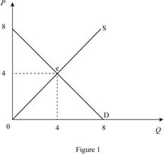
In Figure 1, horizontal axis measures quantity and vertical axis measures price. The curve D indicates demand and the curve S indicates supply. Market reaches the equilibrium at point ‘e’ where the demand curve intersects with supply curve.
Equilibrium price can be calculated as follows.
Equilibrium price is $4.
Thus, equilibrium quantity is 4 units.
Consumer surplus is $8.
Producer surplus is $8.
Total surplus can be calculated as follows.
Total surplus is $16.
Concept introduction:
Consumer surplus: It is the difference between the highest willing price of the consumer and the actual price that the consumer pays.
Producer surplus: It is the difference between the minimum accepted price for the producer and the actual price received by the producer.
Equilibrium price: It is the market price determined by equating the supply to the demand. At this equilibrium point, the supply will be equal to the demand and there will be no excess demand or
Subpart (b):
The equilibrium price and the quantity of haircuts and total surplus.
Subpart (b):
Explanation of Solution
The world price for the good is $1. Thus, when the country opens the market for trade, the price becomes $1 in domestic country too. Figure 2 describe this situation.
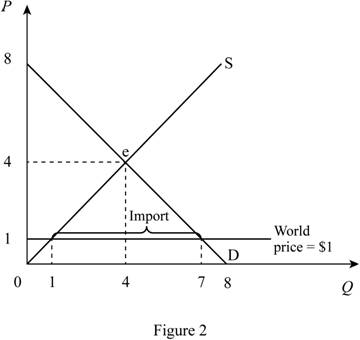
In Figure 2, horizontal axis measures quantity and vertical axis measures price. The curve D indicates demand and the curve S indicates supply. Market reaches the equilibrium at point ‘e’ where the demand curve intersects with supply curve.
When the competitor (Rest of the world) sells a good at price $1, in domestic country equilibrium price become equal to world price. Thus, equilibrium price in the domestic country is $1.
Equilibrium domestic supply can be calculated by substituting the domestic equilibrium price in to supply equation.
Thus, equilibrium quantity is 1 unit.
Equilibrium domestic demand can be calculated by substituting the domestic equilibrium price in to demand equation.
Thus, equilibrium domestic demand is 7 units.
Total imports can be calculated as follows.
Domestic imports are 6 units.
Consumer surplus can be calculated as follows.
Consumer surplus is $24.5.
Producer surplus can be calculated as follows.
Producer surplus is $0.5.
Total surplus can be calculated as follows.
Total surplus is $25.
Concept introduction:
Consumer surplus: It is the difference between the highest willing price of the consumer and the actual price that the consumer pays.
Producer surplus: It is the difference between the minimum accepted price for the producer and the actual price received by the producer.
Equilibrium price: It is the market price determined by equating the supply to the demand. At this equilibrium point, the supply will be equal to the demand and there will be no excess demand or excess supply in an economy. Thus, the economy will be at equilibrium.
Subpar (c):
The equilibrium price and the quantity of haircuts and total surplus.
Subpar (c):
Explanation of Solution
When domestic country impose tariff of $1, the price in domestic country increases from $1 to $2. This increase in price is shown in the Figure 3.
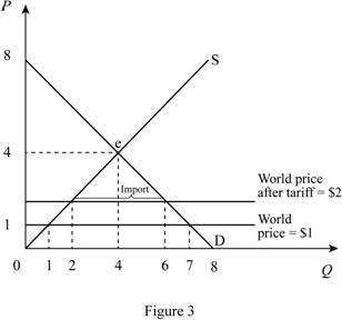
In Figure 3, horizontal axis measures quantity and vertical axis measures price. The curve D indicates demand and the curve S indicates supply. Market reaches the equilibrium at point ‘e’ where the demand curve intersects with supply curve. Price is increases from $1 to $2 due to the tariff of $1.
Domestic equilibrium price can be calculated as follows.
New domestic price is $2.
Equilibrium domestic supply can be calculated by substituting the domestic equilibrium price in to supply equation.
Thus, equilibrium quantity is 2 units.
Equilibrium domestic demand can be calculated by substituting the domestic equilibrium price in to demand equation.
Thus, equilibrium domestic demand is 6 units.
Total imports can be calculated as follows.
Domestic imports are 4 units.
Consumer surplus can be calculated as follows.
Consumer surplus is $18.
Producer surplus can be calculated as follows.
Producer surplus is $2.
Government revenue can be calculated as follows.
Government revenue is 4.
Total surplus can be calculated as follows.
Total surplus is $24.
Concept introduction:
Consumer surplus: It is the difference between the highest willing price of the consumer and the actual price that the consumer pays.
Producer surplus: It is the difference between the minimum accepted price for the producer and the actual price received by the producer.
Equilibrium price: It is the market price determined by equating the supply to the demand. At this equilibrium point, the supply will be equal to the demand and there will be no excess demand or excess supply in an economy. Thus, the economy will be at equilibrium.
Subpart (d):
Calculate total gains and
Subpart (d):
Explanation of Solution
Total gains from opening up trade can be calculated as follows.
Total gains are$8.
Deadweight loss can be calculated as follows.
Deadweight loss is $1.
Want to see more full solutions like this?
Chapter 9 Solutions
Principles of Macroeconomics (MindTap Course List)

- How does the change in consumer and producer surplus compare with the tax revenue?arrow_forwardConsidering the following supply and demand equations: Qs=3P-1 Qd=-2P+9 dPdt=0.5(Qd-Qs) Find the expressions: P(t), Qs(t) and Qd(t). When P(0)=1, is the system stable or unstable? If the constant for the change of excess of demand changes to 0.6, this is: dPdt=0.6(Qd-Qs) do P(t), Qs(t) and Qd(t) remain the same when P(0)=1?arrow_forwardConsider the following supply and demand schedule of wooden tables.a. Draw the corresponding graphs for supply and demand. b. Using the data, obtain the corresponding supply and demand functions. c. Find the market-clearing price and quantity. Price (Thousands USD) Supply Demand2 96 1104 196 1906 296 270 8 396 35010 496 43012 596 51014 696 59016 796 67018 896 75020 996 830arrow_forward
- What happens to consumer surplus and producer surplus when the sale of a good is taxed?arrow_forwardEconomics Grade 3 CONDUCT RESEARCH ON (the various) MARKET STRUCTURES Research Project/May Explain the concept market structure and explain why there are perfect and imperfect market structures. (5) • Provide reasons as to why the taxi industry is regarded as operating in a monopolistic competitive structure. (10) • How do monopolies impact consumers and the economy. (10) • Use graph(s) to explain the long run equilibrium price and output in a perfect market. (10) • Evaluate the effectiveness of South Africa's competition policy in curbing anticompetitive tendencies in the market. Make use of practical examples. (10) GRAND TOTAL:50 Please turn Copyrightarrow_forwardUGD KCQ 2: Microeconomic Essentials (page 11 of 20) - Google Chrome mancosaconnect.ac.za/mod/quiz/attempt.php?attempt=1958913&cmid=436375&page=10 MANCOSA Microeconomic Essentials Jan25 Y1 S1 Back Refer to the diagram below to answer the question that follows: Price PH P1 D₁ ㅁ X Quiz navigation 3 4 5 6 Time left 0:58:34 1 2 Question 11 7 8 Not yet answered Marked out of 1.00 13 33 14 S₁ Flag question Q Q1 Quantity Which of the following may result in a shift of the supply curve from S to S1? OA. An increase in price of the good. B. An increase in wages. O C. A decrease in price of the good. O D. An improvement in the technique of production. https://mancosaconnect.ac.za/mod/quiz/attempt.php?attempt=1958913&cmid=436375&page=10#question-2064270-11 19 20 6 10 10 11 12 15 Question 11- Not yet answered Finish attempt... 7:31 PMarrow_forward
- Euros per U.S. Doler Consider the model below, showing the supply and demand curves for the exchange market of U.S. Dollars and Euros. If the inflation rate in the U.S. increases (and in the European Union stays the same), how will that change the original equilibrium shown in the graph? 1.10- 1.00- 0.90 0.80- 0.70 0.60 0.50- 0.40- 0.30 0.20 E 4.7 48 49 50 51 52 53 54 55 56 Quantity of U.S. Dollars traded for Euros (trillionsday) O It will decrease the demand for Dollars and increase the supply, so the exchange rate decreases and the impact on the quantity traded is unknown. O It will decrease the demand for Dollars and increase the supply, so the exchange rate decreases, and the quantity traded increases. It will increase the demand for Dollars and decrease the supply, so the exchange rate decreases, and the quantity traded increases. It will increase the demand for Dollars and decrease the supply, so the exchange rate increases and the impact on the quantity traded is unknownarrow_forwardIf the US Federal Reserve increases interests on reserves, how will that change the original equilibrium shown in the graph? Euros par US alar 1.10 1.00 0.90- E 0.80- 0.70 0.60 0.50 0.40- 0.30 0.20 47 48 49 50 51 52 53 54 55 56 Quantity of US Dollars traded for Euros (trillions/day) It will increase the demand for Dollars and decrease the supply, so the exchange rate decreases, and the quantity traded increases. O It will decrease the demand for Dollars and increase the supply, so the exchange rate decreases and the impact on the quantity traded is unknown. O It will increase the demand for Dollars and decrease the supply, so the exchange rate increases and the impact on the quantity traded is unknown O It will decrease the demand for Dollars and increase the supply, so the exchange rate decreases, and the quantity traded increases. Question 22 5 ptsarrow_forward1. Based on the video, answer the following questions. • What are the 5 key characteristics that differentiate perfect competition from monopoly? Based on the video. • How does the number of sellers in a market influence the type of market structure? Based on the video. • In what ways does product differentiation play a role in monopolistic competition? Based on the video. • How do barriers to entry affect the level of competition in an oligopoly? Based on the video. • Why might firms in an oligopolistic market engage in non-price competition rather than price wars? Based on the video. Reference video: https://youtu.be/Qrr-IGR1kvE?si=h4q2F1JFNoCI36TVarrow_forward
- 1. Answer the following questions based on the reference video below: • What are the 5 key characteristics that differentiate perfect competition from monopoly? • How does the number of sellers in a market influence the type of market structure? • In what ways does product differentiation play a role in monopolistic competition? • How do barriers to entry affect the level of competition in an oligopoly? • Why might firms in an oligopolistic market engage in non-price competition rather than price wars? Discuss. Reference video: https://youtu.be/Qrr-IGR1kvE?si=h4q2F1JFNoCI36TVarrow_forwardExplain the importance of differential calculus within economics and business analysis. Provide three refernces with your answer. They can be from websites or a journals.arrow_forwardAnalyze the graph below, showing the Gross Federal Debt as a percentage of GDP for the United States (1939-2019). Which of the following is correct? FRED Gross Federal Debt as Percent of Gross Domestic Product Percent of GDP 120 110 100 60 50 40 90 30 1940 1950 1960 1970 Shaded areas indicate US recessions 1980 1990 2000 2010 1000 Sources: OMD, St. Louis Fed myfred/g/U In 2019, the Federal Government of the United States had an accumulated debt/GDP higher than 100%, meaning that the amount of debt accumulated over time is higher than the value of all goods and services produced in that year. The debt/GDP is always positive during this period, so the Federal Government of the United States incurred in budget deficits every year since 1939. From the mid-40s until the mid-70s, the debt/DGP was decreasing, meaning that the Federal Government of the United States was running a budget surplus every year during those three decades. During the second half of the 1970s, the Federal Government…arrow_forward
 Principles of MicroeconomicsEconomicsISBN:9781305156050Author:N. Gregory MankiwPublisher:Cengage Learning
 Principles of Economics, 7th Edition (MindTap Cou...EconomicsISBN:9781285165875Author:N. Gregory MankiwPublisher:Cengage Learning
 Principles of Macroeconomics (MindTap Course List)EconomicsISBN:9781285165912Author:N. Gregory MankiwPublisher:Cengage Learning
 Microeconomics: Private and Public Choice (MindTa...EconomicsISBN:9781305506893Author:James D. Gwartney, Richard L. Stroup, Russell S. Sobel, David A. MacphersonPublisher:Cengage Learning
 Macroeconomics: Private and Public Choice (MindTa...EconomicsISBN:9781305506756Author:James D. Gwartney, Richard L. Stroup, Russell S. Sobel, David A. MacphersonPublisher:Cengage Learning
 Economics: Private and Public Choice (MindTap Cou...EconomicsISBN:9781305506725Author:James D. Gwartney, Richard L. Stroup, Russell S. Sobel, David A. MacphersonPublisher:Cengage Learning