
Subpart (a):
Calculate different costs.
Subpart (a):
Explanation of Solution
Total cost (TC) can be obtained by using the following formula.
Total cost at production level 1 unit can be calculated by substituting the respective values in Equation (1).
Total cost is $105.
Average fixed cost (AFC) can be obtained by using the following formula.
Average fixed cost at production level 1 unit can be calculated by substituting the respective values in Equation (2).
Average fixed cost is $60.
Average variable cost at production level 1 unit can be calculated by substituting the respective values in Equation (3).
Average variable cost is $45.
Total average cost (AC) can be obtained by using the following formula.
Total average cost at production level 1 unit can be calculated by substituting the respective values in Equation (4).
Average variable cost is $105.
Marginal cost (MC) can be obtained by using the following formula.
Average variable cost at production level 1 unit can be calculated by substituting the respective values in Equation (5).
Marginal cost is $105.
Table-1 shows the total cost, average fixed cost, average variable cost,
Table -1
| Quantity | Fixed cost | Variable cost | TC | AFC | AVC | AC | MC |
| 0 | 60 | 0 | 60 | ||||
| 1 | 60 | 45 | 105 | 60 | 45.00 | 105.00 | 45 |
| 2 | 60 | 85 | 145 | 30 | 42.50 | 72.50 | 40 |
| 3 | 60 | 120 | 180 | 20 | 40.00 | 60.00 | 35 |
| 4 | 60 | 150 | 210 | 15 | 37.50 | 52.50 | 30 |
| 5 | 60 | 185 | 245 | 12 | 37.00 | 49.00 | 35 |
| 6 | 60 | 225 | 285 | 10 | 37.50 | 47.50 | 40 |
| 7 | 60 | 270 | 330 | 8.57 | 38.57 | 47.14 | 45 |
| 8 | 60 | 325 | 385 | 7.50 | 40.63 | 48.13 | 55 |
| 9 | 60 | 390 | 450 | 6.67 | 43.33 | 50.00 | 65 |
| 10 | 60 | 465 | 525 | 6 | 46.50 | 52.50 | 75 |
Figure -1 illustrates the shape of total fixed cost, total cost and total variable cost that influencing by the diminishing returns to scale.
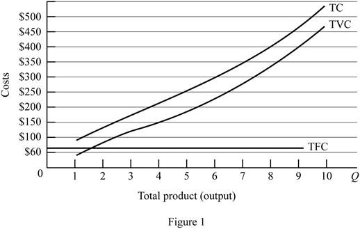
In figure -1, horizontal axis measures total output and vertical axis measures cost. The curve TC indicates total cost and the curve TVC indicates total variable cost. TFC curve indicates total fixed cost. Since total fixed cost is remain the same over the different level of production TFC curve parallel to the horizontal axis.
From the output range 1 unit to 4 units, total cost and total variable cost increasing at decreasing rate due to the increasing marginal returns. Thereafter, these two cost curves are increasing at increasing rate due to the diminishing marginal cost.
Concept introduction:
Fixed cost: Fixed costs refer to those costs that remain the same regardless of the level of production.
Variable cost: Variable cost refers to the costs that change due to the changes occurring in the level of production.
Subpart (b):
Calculate different costs.
Subpart (b):
Explanation of Solution
Figure -2 illustrates relationship between marginal cost, average variable cost, average fixed cost and average total cost curve.
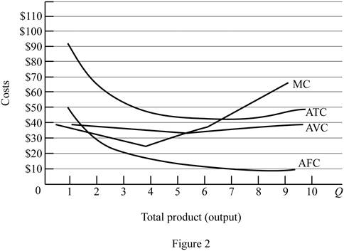
In figure -2, horizontal axis measures total output and vertical axis measures cost. The curve TC indicates total cost and the curve TVC indicates total variable cost. TFC curve indicates total fixed cost. Since total fixed cost is remain the same over the different level of production TFC curve parallel to the horizontal axis.
Since the fixed cost is spread over all the output, increasing the level of output leads to reduce the average fixed cost over the increasing production. Marginal cost curve average variable cost curve and average total cost curve are U shaped due to the operation of economies of scale and diseconomies of scale.
Average total cost curve is the vertical summation of average fixed cost and average variable cost. When the marginal cost curve is below to the average total cost curve, then the average total cost falls. When the marginal cost lies above the average total cost curve then the average total cost curve start rises. Thus, marginal cost curve intersects with the average total cost curve at the minimum point.
When the marginal cost curve is below to the average variable cost curve, then the average variable cost falls. When the marginal cost lies above the average variable cost curve then the average variable cost curve start rises. Thus, marginal cost curve intersects with the average variable cost curve at the minimum point.
Concept introduction:
Fixed cost: Fixed costs refer to those costs that remain the same regardless of the level of production.
Variable cost: Variable cost refers to the costs that change due to the changes occurring in the level of production.
Subpart (c):
Fixed cost and variable cost.
Subpart (c):
Explanation of Solution
The increasing fixed cost from $60 to $100 leads to shifts the fixed cost curve upward (By $40). This increasing fixed cost does not affect the marginal cost. Thus, marginal cost curve and average variable cost curve remains the same.
The decrease in variable cost by $10 leads to reduce the marginal cost $10 at first level of output and remains the same for other level of output. Average total cost and average variable cost decreases as a result of decrease in the variable cost. But, average fixed cost remains the same.
Concept introduction:
Fixed cost: Fixed costs refer to those costs that remain the same regardless of the level of production.
Variable cost: Variable cost refers to the costs that change due to the changes occurring in the level of production.
Want to see more full solutions like this?
Chapter 9 Solutions
EP ECONOMICS,AP EDITION-CONNECT ACCESS

- How did Jennifer Lopez use free enterprise to become successful ?arrow_forwardAn actuary analyzes a company’s annual personal auto claims, M and annual commercialauto claims, N . The analysis reveals that V ar(M ) = 1600, V ar(N ) = 900, and thecorrelation between M and N is ρ = 0.64. Compute V ar(M + N ).arrow_forwardDon't used hand raitingarrow_forward
- Answer in step by step with explanation. Don't use Ai.arrow_forwardUse the figure below to answer the following question. Let I represent Income when healthy, let I represent income when ill. Let E [I] represent expected income for a given probability (p) of falling ill. Utility у в ULI income Is есте IM The actuarially fair & partial contract is represented by Point X × OB A Yarrow_forwardSuppose that there is a 25% chance Riju is injured and earns $180,000, and a 75% chance she stays healthy and will earn $900,000. Suppose further that her utility function is the following: U = (Income) ³. Riju's utility if she earns $180,000 is _ and her utility if she earns $900,000 is. X 56.46; 169.38 56.46; 96.55 96.55; 56.46 40.00; 200.00 169.38; 56.46arrow_forward
- Use the figure below to answer the following question. Let là represent Income when healthy, let Is represent income when ill. Let E[I], represent expected income for a given probability (p) of falling ill. Utility & B естве IH S Point D represents ☑ actuarially fair & full contract actuarially fair & partial contract O actuarially unfair & full contract uninsurance incomearrow_forwardSuppose that there is a 25% chance Riju is injured and earns $180,000, and a 75% chance she stays healthy and will earn $900,000. Suppose further that her utility function is the following: U = (Income). Riju is risk. She will prefer (given the same expected income). averse; no insurance to actuarially fair and full insurance lover; actuarially fair and full insurance to no insurance averse; actuarially fair and full insurance to no insurance neutral; he will be indifferent between actuarially fair and full insurance to no insurance lover; no insurance to actuarially fair and full insurancearrow_forward19. (20 points in total) Suppose that the market demand curve is p = 80 - 8Qd, where p is the price per unit and Qd is the number of units demanded per week, and the market supply curve is p = 5+7Qs, where Q5 is the quantity supplied per week. a. b. C. d. e. Calculate the equilibrium price and quantity for a competitive market in which there is no market failure. Draw a diagram that includes the demand and supply curves, the values of the vertical- axis intercepts, and the competitive equilibrium quantity and price. Label the curves, axes and areas. Calculate both the marginal willingness to pay and the total willingness to pay for the equilibrium quantity. Calculate both the marginal cost of the equilibrium quantity and variable cost of producing the equilibrium quantity. Calculate the total surplus. How is the value of total surplus related to your calculations in parts c and d?arrow_forward

 Economics (MindTap Course List)EconomicsISBN:9781337617383Author:Roger A. ArnoldPublisher:Cengage Learning


 Principles of Economics 2eEconomicsISBN:9781947172364Author:Steven A. Greenlaw; David ShapiroPublisher:OpenStax