
To find:
A 99% confidence interval for the mean
Answer to Problem 14E
Solution:
A 99% confidence interval for the mean face amount of an individual life insurance policy is in the interval,
Explanation of Solution
Approach:
Given a sample with standard deviation
The true population parameters probability lies in this interval range which is known as the confidence level
At a certain level of confidence, the interval in which the maximum error can be observed is known as the confidence interval.
Estimating parameters of a large population or a population following
The
The degrees of freedom is the attribute used to obtain the appropriate curve for the
The value of
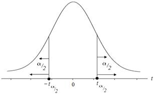
Hence this is a case of two-tailed t-distribution.
The maximum distance from point estimate that the confidence interval covers is margin of error and is given by:
Given the sample mean
Calculation:
The sample means is given by:
Substituting the values of life insurance policies in the formula above
| 150, 000 | 171758.62 | -21, 758.62 | 473437544.3 |
| 150, 000 | 171758.62 | -21, 758.62 | 473437544.3 |
| 150, 000 | 171758.62 | -21, 758.62 | 473437544.3 |
| 150, 000 | 171758.62 | -21, 758.62 | 473437544.3 |
| 150, 000 | 171758.62 | -21, 758.62 | 473437544.3 |
| 150, 000 | 171758.62 | -21, 758.62 | 473437544.3 |
| 151, 000 | 171758.62 | -20, 758.62 | 430920304.3 |
| 152, 000 | 171758.62 | -19, 758.62 | 390403064.3 |
| 152, 000 | 171758.62 | -19, 758.62 | 390403064.3 |
| 153, 000 | 171758.62 | -18, 758.62 | 351885824.3 |
| 153, 000 | 171758.62 | -18, 758.62 | 351885824.3 |
| 154, 000 | 171758.62 | -17, 758.62 | 315368584.3 |
| 155, 000 | 171758.62 | -16, 758.62 | 280851344.3 |
| 158, 000 | 171758.62 | -13, 758.62 | 189299624.3 |
| 158, 000 | 171758.62 | -12, 758.62 | 162782384.3 |
| 158, 000 | 171758.62 | -12, 758.62 | 162782384.3 |
| 160, 000 | 171758.62 | -11, 758.62 | 138265144.3 |
| 160, 000 | 171758.62 | -11, 758.62 | 138265144.3 |
| 160, 000 | 171758.62 | -11, 758.62 | 138265144.3 |
| 162, 000 | 171758.62 | -9, 758.62 | 95230664.3 |
| 163, 000 | 171758.62 | -8, 758.62 | 76713424.3 |
| 163, 000 | 171758.62 | -8, 758.62 | 76713424.3 |
| 163, 000 | 171758.62 | -8, 758.62 | 76713424.3 |
| 165, 000 | 171758.62 | -6, 758.62 | 45678944.3 |
| 165, 000 | 171758.62 | -6, 758.62 | 45678944.3 |
| 168, 000 | 171758.62 | -3, 758.62 | 14127224.3 |
| 168, 000 | 171758.62 | -3, 758.62 | 14127224.3 |
| 168, 000 | 171758.62 | -3, 758.62 | 14127224.3 |
| 171, 000 | 171758.62 | -758.62 | 575504.3044 |
| 171, 000 | 171758.62 | -758.62 | 575504.3044 |
| 172, 000 | 171758.62 | 241.38 | 58264.3044 |
| 172, 000 | 171758.62 | 241.38 | 58264.3044 |
| 172, 000 | 171758.62 | 241.38 | 58264.3044 |
| 173, 000 | 171758.62 | 1, 241.38 | 1541024.304 |
| 174, 000 | 171758.62 | 2, 241.38 | 5023784.304 |
| 175, 000 | 171758.62 | 3, 241.38 | 10506544.3 |
| 175, 000 | 171758.62 | 3, 241.38 | 10506544.3 |
| 175, 000 | 171758.62 | 3, 241.38 | 10506544.3 |
| 176, 000 | 171758.62 | 4, 241.38 | 17989304.3 |
| 182, 000 | 171758.62 | 10, 241.38 | 104885864.3 |
| 182, 000 | 171758.62 | 10, 241.38 | 104885864.3 |
| 183, 000 | 171758.62 | 11, 241.38 | 126368624.3 |
| 185, 000 | 171758.62 | 13, 241.38 | 175334144.3 |
| 185, 000 | 171758.62 | 13, 241.38 | 175334144.3 |
| 190, 000 | 171758.62 | 18, 241.38 | 332747944.3 |
| 190, 000 | 171758.62 | 18, 241.38 | 332747944.3 |
| 195, 000 | 171758.62 | 23, 241.38 | 540161744.3 |
| 195, 000 | 171758.62 | 23, 241.38 | 540161744.3 |
| 195, 000 | 171758.62 | 23, 241.38 | 540161744.3 |
| 196, 000 | 171758.62 | 24, 241.38 | 587644504.3 |
| 200, 000 | 171758.62 | 28, 241.38 | 797575544.3 |
| 200, 000 | 171758.62 | 28, 241.38 | 797575544.3 |
| 200, 000 | 171758.62 | 28, 241.38 | 797575544.3 |
| 200, 000 | 171758.62 | 28, 241.38 | 797575544.3 |
| 200, 000 | 171758.62 | 28, 241.38 | 797575544.3 |
| 202, 000 | 171758.62 | 30, 241.38 | 914541064.3 |
| 202, 000 | 171758.62 | 30, 241.38 | 914541064.3 |
| 163, 000 | 171758.62 | -8, 758.62 | 76713424.3 |
Form the above table we get,
Now the standard division is,
Level of confidence is 99%
Where
Critical t value at
Now substitute these values in margin of error.
Then, the margin of error is calculated as:
Then, interval is:
Conclusion:
A 95% confidence interval for the mean fastball pitching speed of all high school is in the interval
Want to see more full solutions like this?
Chapter 8 Solutions
Beginning Statistics, 2nd Edition

- Business Discussarrow_forwardThe following data represent total ventilation measured in liters of air per minute per square meter of body area for two independent (and randomly chosen) samples. Analyze these data using the appropriate non-parametric hypothesis testarrow_forwardeach column represents before & after measurements on the same individual. Analyze with the appropriate non-parametric hypothesis test for a paired design.arrow_forward
- Should you be confident in applying your regression equation to estimate the heart rate of a python at 35°C? Why or why not?arrow_forwardGiven your fitted regression line, what would be the residual for snake #5 (10 C)?arrow_forwardCalculate the 95% confidence interval around your estimate of r using Fisher’s z-transformation. In your final answer, make sure to back-transform to the original units.arrow_forward
 MATLAB: An Introduction with ApplicationsStatisticsISBN:9781119256830Author:Amos GilatPublisher:John Wiley & Sons Inc
 Probability and Statistics for Engineering and th...StatisticsISBN:9781305251809Author:Jay L. DevorePublisher:Cengage Learning
 Statistics for The Behavioral Sciences (MindTap C...StatisticsISBN:9781305504912Author:Frederick J Gravetter, Larry B. WallnauPublisher:Cengage Learning
 Elementary Statistics: Picturing the World (7th E...StatisticsISBN:9780134683416Author:Ron Larson, Betsy FarberPublisher:PEARSON
 The Basic Practice of StatisticsStatisticsISBN:9781319042578Author:David S. Moore, William I. Notz, Michael A. FlignerPublisher:W. H. Freeman
 Introduction to the Practice of StatisticsStatisticsISBN:9781319013387Author:David S. Moore, George P. McCabe, Bruce A. CraigPublisher:W. H. Freeman