
a.
To construct: A plot using the distribution of neuronal response to a pure tone and find the numerical summary. Also check whether there outliers exist or not, if yes then again find the numerical summary by omitting it and explain their influence.
a.
Explanation of Solution
Given:
The dataset:
| Neuron | Tone | Call | Neuron | Tone | Call |
| 1 | 474 | 500 | 20 | 100 | 118 |
| 2 | 256 | 138 | 21 | 74 | 62 |
| 3 | 241 | 485 | 22 | 72 | 112 |
| 4 | 226 | 338 | 23 | 20 | 193 |
| 5 | 185 | 194 | 24 | 21 | 129 |
| 6 | 174 | 159 | 25 | 26 | 135 |
| 7 | 176 | 341 | 26 | 71 | 134 |
| 8 | 168 | 85 | 27 | 68 | 65 |
| 9 | 161 | 303 | 28 | 59 | 182 |
| 10 | 150 | 208 | 29 | 59 | 97 |
| 11 | 19 | 66 | 30 | 57 | 318 |
| 12 | 20 | 54 | 31 | 56 | 201 |
| 13 | 35 | 103 | 32 | 47 | 279 |
| 14 | 145 | 42 | 33 | 46 | 62 |
| 15 | 141 | 241 | 34 | 41 | 84 |
| 16 | 129 | 194 | 35 | 26 | 203 |
| 17 | 113 | 123 | 36 | 28 | 192 |
| 18 | 112 | 182 | 37 | 31 | 70 |
| 19 | 102 | 141 |
Formula used:
The formula to compute the
Graph:
The
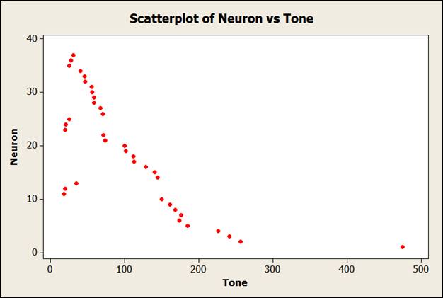
Interpretation:
From the above scatter plot, it is clear that the value 474 is an outlier because it is far distant from the other values.
Calculation:
The numerical summary is:
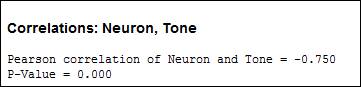
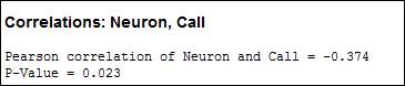
After removal of outlier, the value of the correlation is:
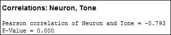
From above output, it is clear that omission of outlier has led the reduction in the value of correlation between the two variables
b.
To construct: A plot using the distribution of neuronal response to a monkey call and find the numerical summary. Also check whether there outliers exist or not, if yes then again find the numerical summary by omitting it and explain their influence.
b.
Explanation of Solution
Graph:
The scatter plot could be constructed as:
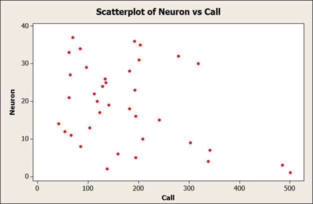
Interpretation:
From the above scatter plot, it is clear that the values 484 and 500 are outlier because they are far distant from the other values.
Calculation:
The numerical summary is:
After removal of outlier, the value of the correlation is:
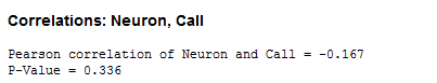
From above output, it is clear that omission of outlier has led increase in the value of correlation between the two variables
c.
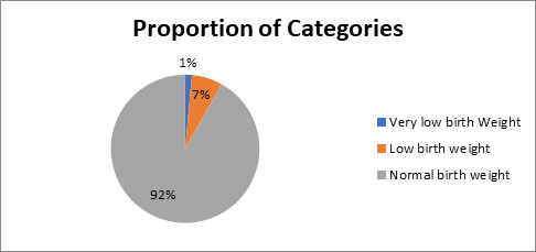
To construct the pie chart or bar chart to show the proportion of given categories.
c.
Explanation of Solution
Given:
The categories:
Very low birth weight: Less than 1500 grams
Low birth weight: Less than 2500 grams
Normal birth weight: More than 2500 grams
Calculation:
Count of each category:
| Category | Frequency | Proportion |
| Very low birth Weight | 57841 | 0.0144768 |
| Low birth weight | 267722 | 0.0670072 |
| Normal birth weight | 3669859 | 0.918516 |
Graph:
d.
To check: whether there any relationship exists between the variables call and tone response by constructing scatter plot and explain it. Also, compute the numerical summary, if possible.
d.
Explanation of Solution
Graph:
The scatter plot could be constructed as:
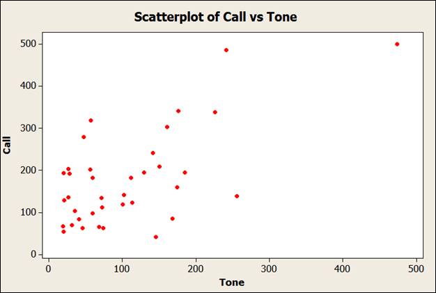
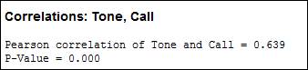
Interpretation:
The above scatter plot shows that there is a
Calculation:
The correlation between the two variables can be calculated as:
Want to see more full solutions like this?
Chapter 8 Solutions
PRACTICE OF STATS - 1 TERM ACCESS CODE

- Need help pleasearrow_forwardPlease conduct a step by step of these statistical tests on separate sheets of Microsoft Excel. If the calculations in Microsoft Excel are incorrect, the null and alternative hypotheses, as well as the conclusions drawn from them, will be meaningless and will not receive any points. 4. One-Way ANOVA: Analyze the customer satisfaction scores across four different product categories to determine if there is a significant difference in means. (Hints: The null can be about maintaining status-quo or no difference among groups) H0 = H1=arrow_forwardPlease conduct a step by step of these statistical tests on separate sheets of Microsoft Excel. If the calculations in Microsoft Excel are incorrect, the null and alternative hypotheses, as well as the conclusions drawn from them, will be meaningless and will not receive any points 2. Two-Sample T-Test: Compare the average sales revenue of two different regions to determine if there is a significant difference. (Hints: The null can be about maintaining status-quo or no difference among groups; if alternative hypothesis is non-directional use the two-tailed p-value from excel file to make a decision about rejecting or not rejecting null) H0 = H1=arrow_forward
- Please conduct a step by step of these statistical tests on separate sheets of Microsoft Excel. If the calculations in Microsoft Excel are incorrect, the null and alternative hypotheses, as well as the conclusions drawn from them, will be meaningless and will not receive any points 3. Paired T-Test: A company implemented a training program to improve employee performance. To evaluate the effectiveness of the program, the company recorded the test scores of 25 employees before and after the training. Determine if the training program is effective in terms of scores of participants before and after the training. (Hints: The null can be about maintaining status-quo or no difference among groups; if alternative hypothesis is non-directional, use the two-tailed p-value from excel file to make a decision about rejecting or not rejecting the null) H0 = H1= Conclusion:arrow_forwardPlease conduct a step by step of these statistical tests on separate sheets of Microsoft Excel. If the calculations in Microsoft Excel are incorrect, the null and alternative hypotheses, as well as the conclusions drawn from them, will be meaningless and will not receive any points. The data for the following questions is provided in Microsoft Excel file on 4 separate sheets. Please conduct these statistical tests on separate sheets of Microsoft Excel. If the calculations in Microsoft Excel are incorrect, the null and alternative hypotheses, as well as the conclusions drawn from them, will be meaningless and will not receive any points. 1. One Sample T-Test: Determine whether the average satisfaction rating of customers for a product is significantly different from a hypothetical mean of 75. (Hints: The null can be about maintaining status-quo or no difference; If your alternative hypothesis is non-directional (e.g., μ≠75), you should use the two-tailed p-value from excel file to…arrow_forwardPlease conduct a step by step of these statistical tests on separate sheets of Microsoft Excel. If the calculations in Microsoft Excel are incorrect, the null and alternative hypotheses, as well as the conclusions drawn from them, will be meaningless and will not receive any points. 1. One Sample T-Test: Determine whether the average satisfaction rating of customers for a product is significantly different from a hypothetical mean of 75. (Hints: The null can be about maintaining status-quo or no difference; If your alternative hypothesis is non-directional (e.g., μ≠75), you should use the two-tailed p-value from excel file to make a decision about rejecting or not rejecting null. If alternative is directional (e.g., μ < 75), you should use the lower-tailed p-value. For alternative hypothesis μ > 75, you should use the upper-tailed p-value.) H0 = H1= Conclusion: The p value from one sample t-test is _______. Since the two-tailed p-value is _______ 2. Two-Sample T-Test:…arrow_forward
- Please conduct a step by step of these statistical tests on separate sheets of Microsoft Excel. If the calculations in Microsoft Excel are incorrect, the null and alternative hypotheses, as well as the conclusions drawn from them, will be meaningless and will not receive any points. What is one sample T-test? Give an example of business application of this test? What is Two-Sample T-Test. Give an example of business application of this test? .What is paired T-test. Give an example of business application of this test? What is one way ANOVA test. Give an example of business application of this test? 1. One Sample T-Test: Determine whether the average satisfaction rating of customers for a product is significantly different from a hypothetical mean of 75. (Hints: The null can be about maintaining status-quo or no difference; If your alternative hypothesis is non-directional (e.g., μ≠75), you should use the two-tailed p-value from excel file to make a decision about rejecting or not…arrow_forwardThe data for the following questions is provided in Microsoft Excel file on 4 separate sheets. Please conduct a step by step of these statistical tests on separate sheets of Microsoft Excel. If the calculations in Microsoft Excel are incorrect, the null and alternative hypotheses, as well as the conclusions drawn from them, will be meaningless and will not receive any points. What is one sample T-test? Give an example of business application of this test? What is Two-Sample T-Test. Give an example of business application of this test? .What is paired T-test. Give an example of business application of this test? What is one way ANOVA test. Give an example of business application of this test? 1. One Sample T-Test: Determine whether the average satisfaction rating of customers for a product is significantly different from a hypothetical mean of 75. (Hints: The null can be about maintaining status-quo or no difference; If your alternative hypothesis is non-directional (e.g., μ≠75), you…arrow_forwardWhat is one sample T-test? Give an example of business application of this test? What is Two-Sample T-Test. Give an example of business application of this test? .What is paired T-test. Give an example of business application of this test? What is one way ANOVA test. Give an example of business application of this test? 1. One Sample T-Test: Determine whether the average satisfaction rating of customers for a product is significantly different from a hypothetical mean of 75. (Hints: The null can be about maintaining status-quo or no difference; If your alternative hypothesis is non-directional (e.g., μ≠75), you should use the two-tailed p-value from excel file to make a decision about rejecting or not rejecting null. If alternative is directional (e.g., μ < 75), you should use the lower-tailed p-value. For alternative hypothesis μ > 75, you should use the upper-tailed p-value.) H0 = H1= Conclusion: The p value from one sample t-test is _______. Since the two-tailed p-value…arrow_forward
- 4. Dynamic regression (adapted from Q10.4 in Hyndman & Athanasopoulos) This exercise concerns aus_accommodation: the total quarterly takings from accommodation and the room occupancy level for hotels, motels, and guest houses in Australia, between January 1998 and June 2016. Total quarterly takings are in millions of Australian dollars. a. Perform inflation adjustment for Takings (using the CPI column), creating a new column in the tsibble called Adj Takings. b. For each state, fit a dynamic regression model of Adj Takings with seasonal dummy variables, a piecewise linear time trend with one knot at 2008 Q1, and ARIMA errors. c. What model was fitted for the state of Victoria? Does the time series exhibit constant seasonality? d. Check that the residuals of the model in c) look like white noise.arrow_forwardce- 216 Answer the following, using the figures and tables from the age versus bone loss data in 2010 Questions 2 and 12: a. For what ages is it reasonable to use the regression line to predict bone loss? b. Interpret the slope in the context of this wolf X problem. y min ball bas oft c. Using the data from the study, can you say that age causes bone loss? srls to sqota bri vo X 1931s aqsini-Y ST.0 0 Isups Iq nsalst ever tom vam noboslios tsb a ti segood insvla villemari aixs-Yediarrow_forward120 110 110 100 90 80 Total Score Scatterplot of Total Score vs. Putts grit bas 70- 20 25 30 35 40 45 50 Puttsarrow_forward
 MATLAB: An Introduction with ApplicationsStatisticsISBN:9781119256830Author:Amos GilatPublisher:John Wiley & Sons Inc
 Probability and Statistics for Engineering and th...StatisticsISBN:9781305251809Author:Jay L. DevorePublisher:Cengage Learning
 Statistics for The Behavioral Sciences (MindTap C...StatisticsISBN:9781305504912Author:Frederick J Gravetter, Larry B. WallnauPublisher:Cengage Learning
 Elementary Statistics: Picturing the World (7th E...StatisticsISBN:9780134683416Author:Ron Larson, Betsy FarberPublisher:PEARSON
 The Basic Practice of StatisticsStatisticsISBN:9781319042578Author:David S. Moore, William I. Notz, Michael A. FlignerPublisher:W. H. Freeman
 Introduction to the Practice of StatisticsStatisticsISBN:9781319013387Author:David S. Moore, George P. McCabe, Bruce A. CraigPublisher:W. H. Freeman