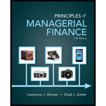
Principles of Managerial Finance (14th Edition) (Pearson Series in Finance)
14th Edition
ISBN: 9780133507690
Author: Lawrence J. Gitman, Chad J. Zutter
Publisher: PEARSON
expand_more
expand_more
format_list_bulleted
Concept explainers
Question
Chapter 8, Problem 8.7P
a)
Summary Introduction
To determine:
Coefficient of variation
Introduction:
The coefficient of variation is an asset risk indicator that measures the relative dispersion. It describes the volatility of asset returns relative to its mean or expected return.
b)
Summary Introduction
To determine:
Alternative recommended to minimize risk.
Introduction:
Risk: The risk can be defined as the uncertainty attached to an event such as investment where there is some amount of risk associated to it as there can be either gain or loss.
The coefficient of variation is an asset risk indicator that measures the relative dispersion. It describes the volatility of asset returns relative to its mean or expected return.
Expert Solution & Answer
Want to see the full answer?
Check out a sample textbook solution
Students have asked these similar questions
Replacement Analysis
The Everly Equipment Company's flange-lipping machine was purchased 5 years ago for $75,000. It had an expected life of 10 years when it was bought and its remaining depreciation is $7,500 per year for each year of its remaining life. As older flange-lippers are robust and useful machines, this one can be sold for $20,000 at the end of its useful life.
A new high-efficiency digital-controlled flange-lipper can be purchased for $130,000, including installation costs. During its 5-year life, it will reduce cash operating expenses by $45,000 per year, although it will not affect sales. At the end of its useful life, the high-efficiency machine is estimated to be worthless. MACRS depreciation will be used, and the machine will be depreciated over its 3-year class life rather than its 5-year economic life, so the applicable depreciation rates are 33.33%, 44.45%, 14.81%, and 7.41%.
The old machine can be sold today for $50,000. The firm's tax rate is 25%, and the…
The Gilbert Instrument Corporation is considering replacing the wood steamer it currently uses to shape guitar sides. The steamer has 6 years of remaining life. If kept, the steamer will have depreciation expenses of $700 for 5 years and $350 for the sixth year. Its current book value is $3,850, and it can be sold on an Internet auction site for $4,440 at this time. If the old steamer is not replaced, it can be sold for $800 at the end of its useful life.
Gilbert is considering purchasing the Side Steamer 3000, a higher-end steamer, which costs $12,300, and has an estimated useful life of 6 years with an estimated salvage value of $1,200. This steamer falls into the MACRS 5-years class, so the applicable depreciation rates are 20.00%, 32.00%, 19.20%, 11.52%, 11.52%, and 5.76%. The new steamer is faster and allows for an output expansion, so sales would rise by $2,000 per year; the new machine's much greater efficiency would reduce operating expenses by $1,800 per year. To support the…
St. Johns River Shipyards' welding machine is 15 years old, fully depreciated, and has no salvage value. However, even though it is old, it is still functional as originally designed and can be used for quite a while longer. A new welder will cost $181,500 and have an estimated life of 8 years with no salvage value. The new welder will be much more efficient, however, and this enhanced efficiency will increase earnings before depreciation from $28,000 to $78,500 per year. The new machine will be depreciated over its 5-year MACRS recovery period, so the applicable depreciation rates are 20.00%, 32.00%, 19.20%, 11.52%, 11.52%, and 5.76%. The applicable corporate tax rate is 25%, and the project cost of capital is 13%. What is the NPV if the firm replaces the old welder with the new one? Do not round intermediate calculations. Round your answer to the nearest dollar. Negative value, if any, should be indicated by a minus sign.
Chapter 8 Solutions
Principles of Managerial Finance (14th Edition) (Pearson Series in Finance)
Ch. 8.1 - Prob. 1FOECh. 8.1 - What is risk in the context of financial decision...Ch. 8.1 - Prob. 8.2RQCh. 8.1 - Prob. 8.3RQCh. 8.2 - Explain how the range is used in scenario...Ch. 8.2 - Prob. 8.5RQCh. 8.2 - Prob. 8.6RQCh. 8.2 - What does the coefficient of variation reveal...Ch. 8.3 - What is an efficient portfolio? How can the return...Ch. 8.3 - Prob. 8.9RQ
Ch. 8.3 - How does international diversification enhance...Ch. 8.4 - Prob. 8.11RQCh. 8.4 - Prob. 8.12RQCh. 8.4 - Prob. 8.13RQCh. 8.4 - What impact would the following changes have on...Ch. 8 - Prob. 1ORCh. 8 - Prob. 8.1STPCh. 8 - Prob. 8.2STPCh. 8 - Prob. 8.1WUECh. 8 - Prob. 8.2WUECh. 8 - Prob. 8.3WUECh. 8 - Prob. 8.4WUECh. 8 - Prob. 8.5WUECh. 8 - Prob. 8.6WUECh. 8 - Prob. 8.1PCh. 8 - Prob. 8.2PCh. 8 - Prob. 8.3PCh. 8 - Prob. 8.4PCh. 8 - Prob. 8.5PCh. 8 - Learning Goal 2 P8-6 Bar charts and risk Swans...Ch. 8 - Prob. 8.7PCh. 8 - Prob. 8.8PCh. 8 - Prob. 8.9PCh. 8 - Prob. 8.10PCh. 8 - Prob. 8.11PCh. 8 - Prob. 8.12PCh. 8 - Prob. 8.13PCh. 8 - Prob. 8.14PCh. 8 - Learning Goal 4 P8- 15 Correlation, risk, and...Ch. 8 - Prob. 8.16PCh. 8 - Learning Goal 5 P8- 17 Total, nondiversifiable,...Ch. 8 - Prob. 8.18PCh. 8 - Prob. 8.19PCh. 8 - Prob. 8.20PCh. 8 - Prob. 8.21PCh. 8 - Prob. 8.22PCh. 8 - Prob. 8.23PCh. 8 - Prob. 8.24PCh. 8 - Prob. 8.25PCh. 8 - Prob. 8.26PCh. 8 - Prob. 8.27PCh. 8 - Learning Goal 6 P8- 28 Security market line (SML)...Ch. 8 - Prob. 8.29PCh. 8 - Prob. 8.30PCh. 8 - Prob. 8.31PCh. 8 - Prob. 1SE
Knowledge Booster
Learn more about
Need a deep-dive on the concept behind this application? Look no further. Learn more about this topic, finance and related others by exploring similar questions and additional content below.Similar questions
- Ends Apr 27 Explain why we start with Sales forecasts when we do our financial forecasting. What are the limitations of the Percent of Sales Forecasting method?arrow_forwardDescribe in detail what exactly is the Cash Conversion Cycle, how is it computed and what is the purpose of this calculation (how is it used).arrow_forwardExplain what Interest Rate Parity is, how it is calculated, and why it is important to a company operating internationally.arrow_forward
- Compare and contrast the three core means of adding shareholder wealth; Cash Dividends, Stock Dividends and Stock Splits, and Stock Repurchases. Include the various advantages and disadvantages of each one.arrow_forwardHow to calculate the future value?arrow_forwardhow to caculate the future value?arrow_forward
- what are some of the question can i asek my prinsiple of finance teache?arrow_forwardA critical discussion of the hockey stick model of start-up financing should be presented, supported by recent in-text citations. Provide a detailed explanation of the model. Describe each of the three stages of the hockey stick model of start-up financing, including a detailed characterisation of each stage. The characterisation of each stage should detail the growth, risk, and funding expectations. Present a critical evaluation and an insightful conclu sion.arrow_forwardQuestion Workspace Check My Work New-Project Analysis The president of your company, MorChuck Enterprises, has asked you to evaluate the proposed acquisition of a new chromatograph for the firm's R&D department. The equipment's basic price is $64,000, and it would cost another $18,000 to modify it for special use by your firm. The chromatograph, which falls into the MACRS 3-year class, would be sold after 3 years for $28,400. The MACRS rates for the first three years are 0.3333, 0.4445 and 0.1481. (Ignore the half-year convention for the straight-line method.) Use of the equipment would require an increase in net working capital (spare parts inventory) of $3,000. The machine would have no effect on revenues, but it is expected to save the firm $24,760 per year in before-tax operating costs, mainly labor. The firm's marginal federal-plus-state tax rate is 25%. Cash outflows and negative NPV value, if any, should be indicated by a minus sign. Do not round intermediate…arrow_forward
arrow_back_ios
SEE MORE QUESTIONS
arrow_forward_ios
Recommended textbooks for you
 Essentials of Business Analytics (MindTap Course ...StatisticsISBN:9781305627734Author:Jeffrey D. Camm, James J. Cochran, Michael J. Fry, Jeffrey W. Ohlmann, David R. AndersonPublisher:Cengage LearningPrinciples of Accounting Volume 2AccountingISBN:9781947172609Author:OpenStaxPublisher:OpenStax College

Essentials of Business Analytics (MindTap Course ...
Statistics
ISBN:9781305627734
Author:Jeffrey D. Camm, James J. Cochran, Michael J. Fry, Jeffrey W. Ohlmann, David R. Anderson
Publisher:Cengage Learning

Principles of Accounting Volume 2
Accounting
ISBN:9781947172609
Author:OpenStax
Publisher:OpenStax College
What is variance analysis?; Author: Corporate finance institute;https://www.youtube.com/watch?v=SMTa1lZu7Qw;License: Standard YouTube License, CC-BY