Concept explainers
Draw the influence lines for the force in member AB, BG, DF, and FG.
Explanation of Solution
Calculation:
Find the support reactions.
Apply 1 k moving load from E to G in the top chord member.
Draw the free body diagram of the member as in Figure 1.
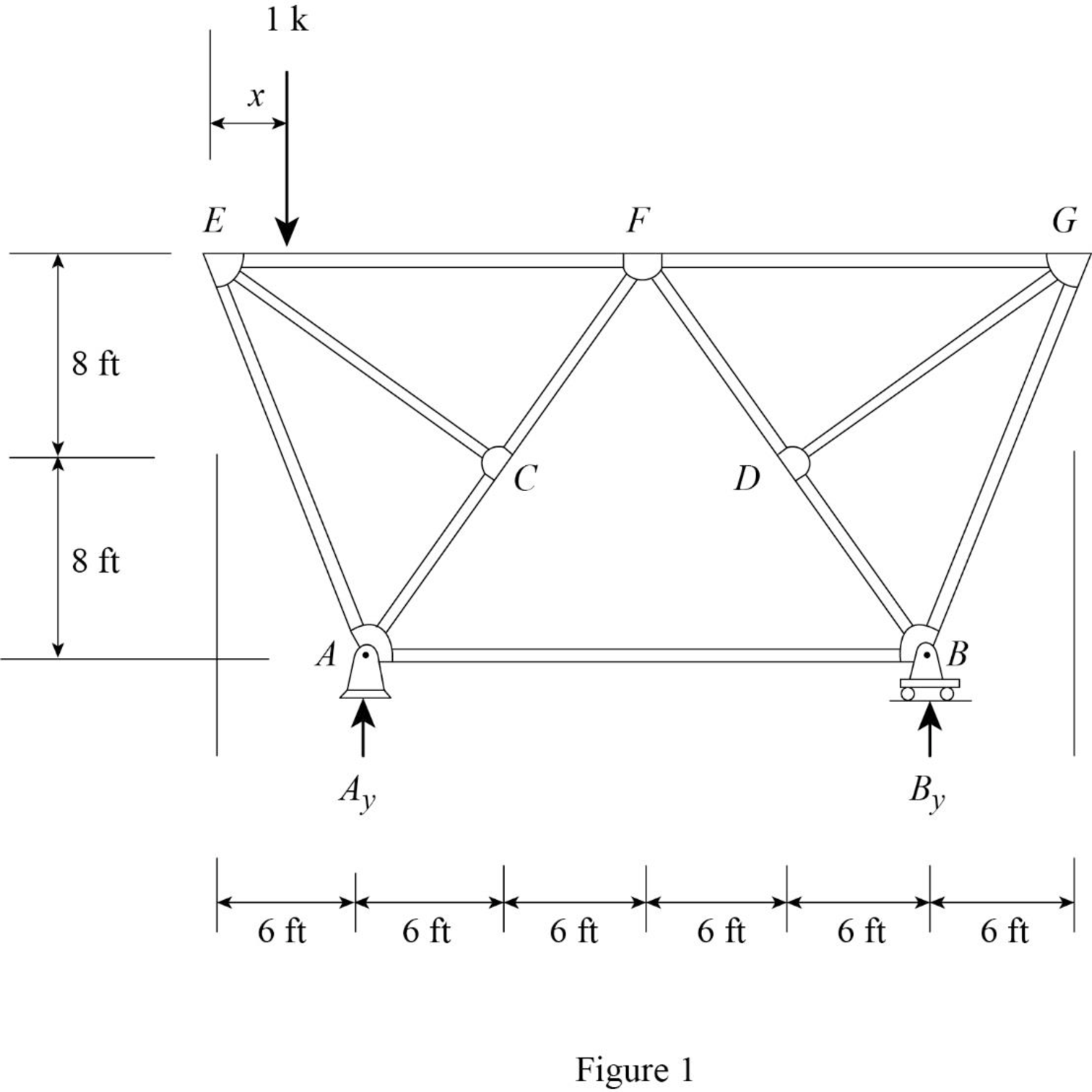
Find the reaction at A and B when 1 k load placed from E to G.
Apply moment equilibrium at A.
Apply force equilibrium equation along vertical.
Consider the upward force as positive
Influence line for the force in member AB.
The expressions for the member force
Draw the free body diagram of member with section aa as shown in Figure 2.
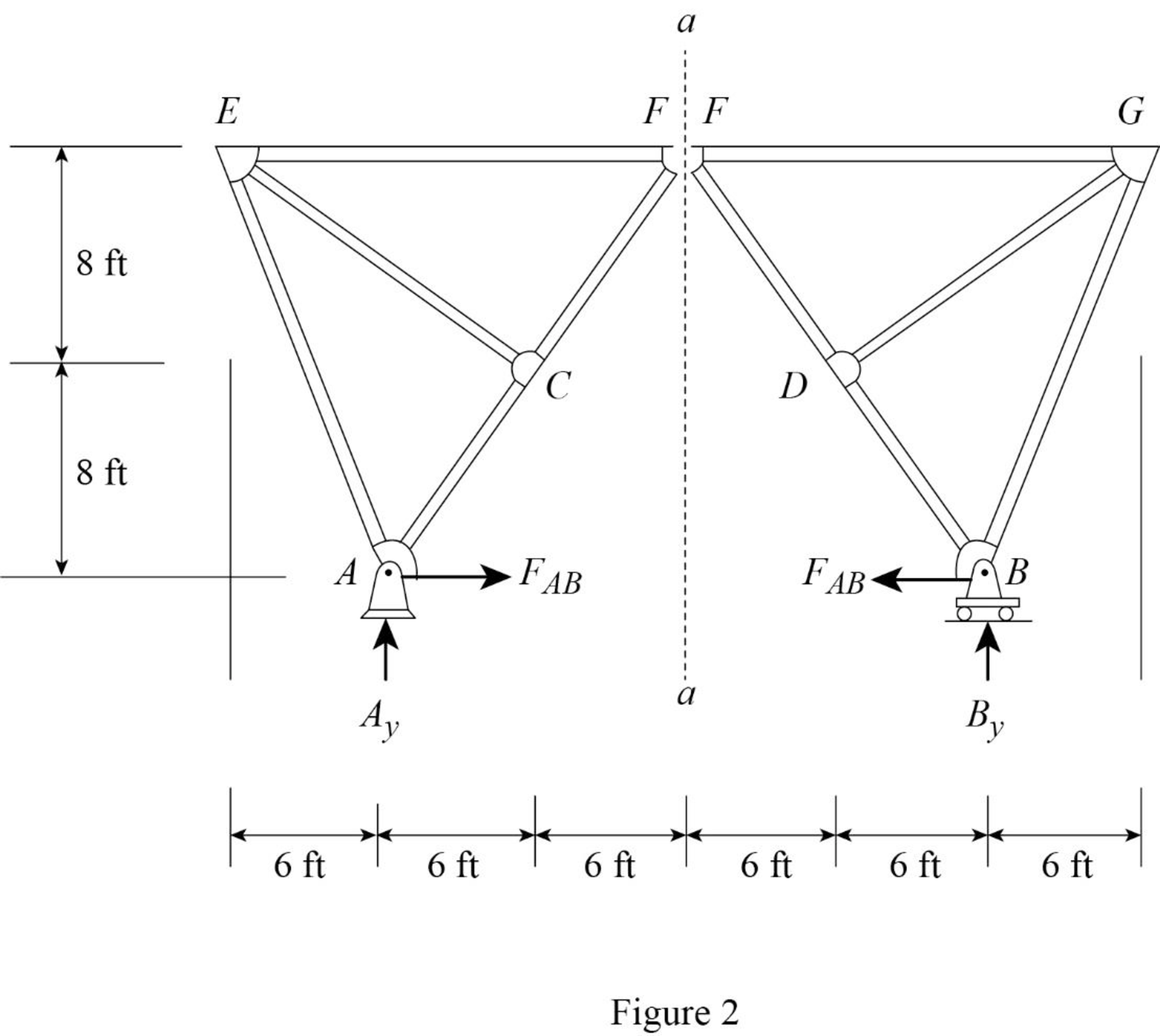
Refer Figure 2.
Find the equation of member force AB.
Apply a 1 k load at just left of F
Consider the right hand portion to section a-a.
Apply moment equilibrium equation at F.
Consider clockwise moment as positive and anticlockwise moment as negative.
Substitute
Apply a 1 k load at just right of F
Consider the left hand portion to section a-a.
Apply moment equilibrium equation at F.
Consider clockwise moment as positive and anticlockwise moment as negative.
Substitute
Thus, the equation of force in the member AB,
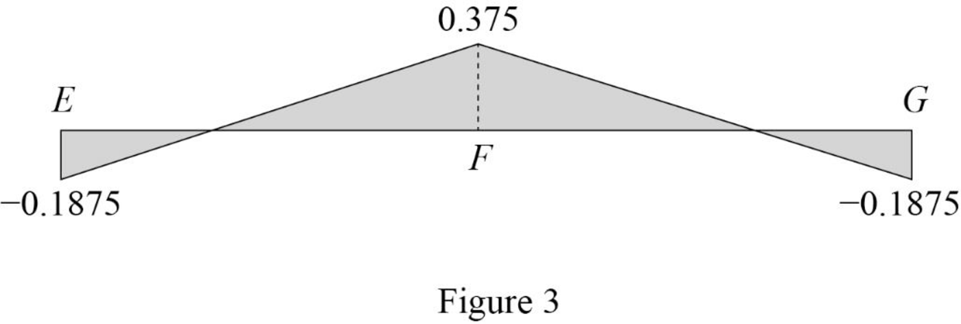
Find the force in member AB using the Equation (1) and (2) and then summarize the value in Table 1.
| x (ft) | Apply 1 k load | Force in member AB (k) | Influence line ordinate for the force in member AB (k/k) |
| 0 | E | ||
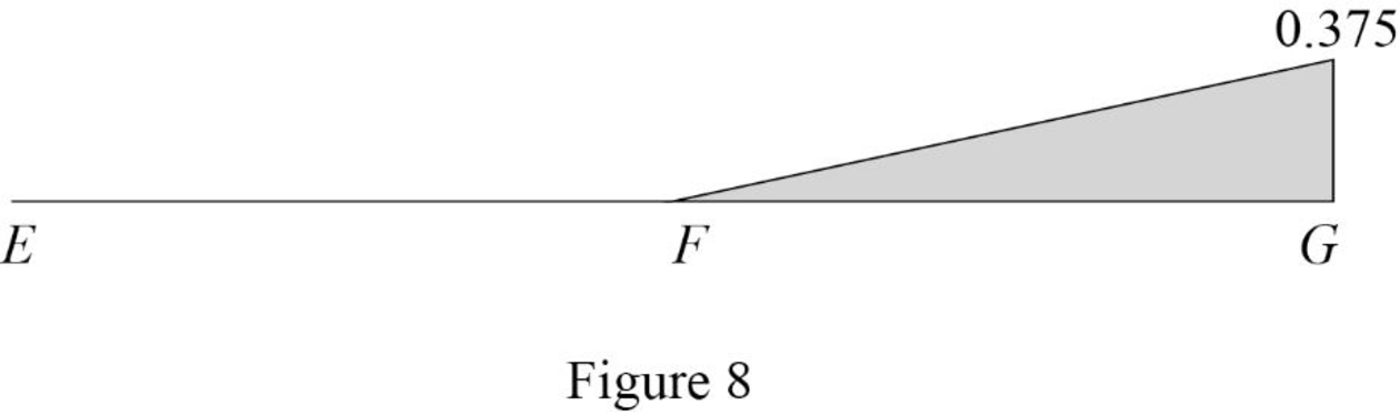
| 18 | F | 0.375 | |
| 36 | G |
Sketch the influence line diagram for ordinate for the force in member AB using Table 2 as shown in Figure 3.
Influence line for the force in member BG.
The expressions for the member force
Draw the free body diagram of section a-a as shown in Figure 4.
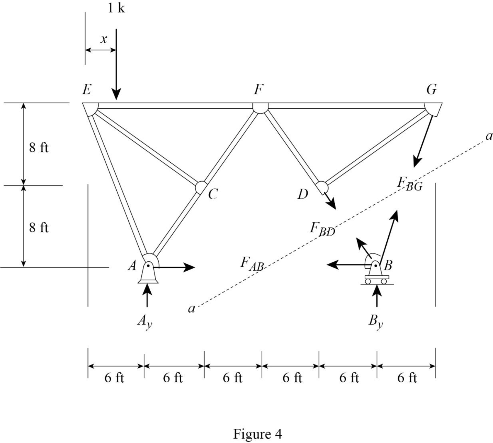
Refer Figure 4.
Find the force in member BG.
Apply 1 k load just left of F
Consider the section EF.
The member force of EF not affected when 1 k load applied from E to F. Therefore, the influence line ordinate of member force BG is 0 k/k from E to F.
Apply a 1 k load just the right of F
Apply moment equilibrium at F.
Consider the section right of line a-a.
Consider clockwise moment as positive and anticlockwise moment as negative.
Substitute
Thus, the equation of force in the member BG,
Find the force in member BG using the Equation (3) and (4) and then summarize the value in Table 2.
| x (ft) | Apply 1 k load | Force in member BG (k) | Influence line ordinate for the force in member BG (k/k) |
| 0 | E | 0 | |
| 18 | F | 0 | |
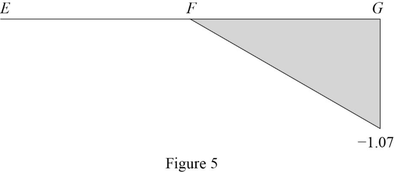
| 36 | G | ‑1.07 |
Sketch the influence line diagram for ordinate for the force in member BG using Table 2 as shown in Figure 5.
Influence line for the force in member DF.
The expressions for the member force
Draw the free body diagram of section a-a as shown in Figure 6.
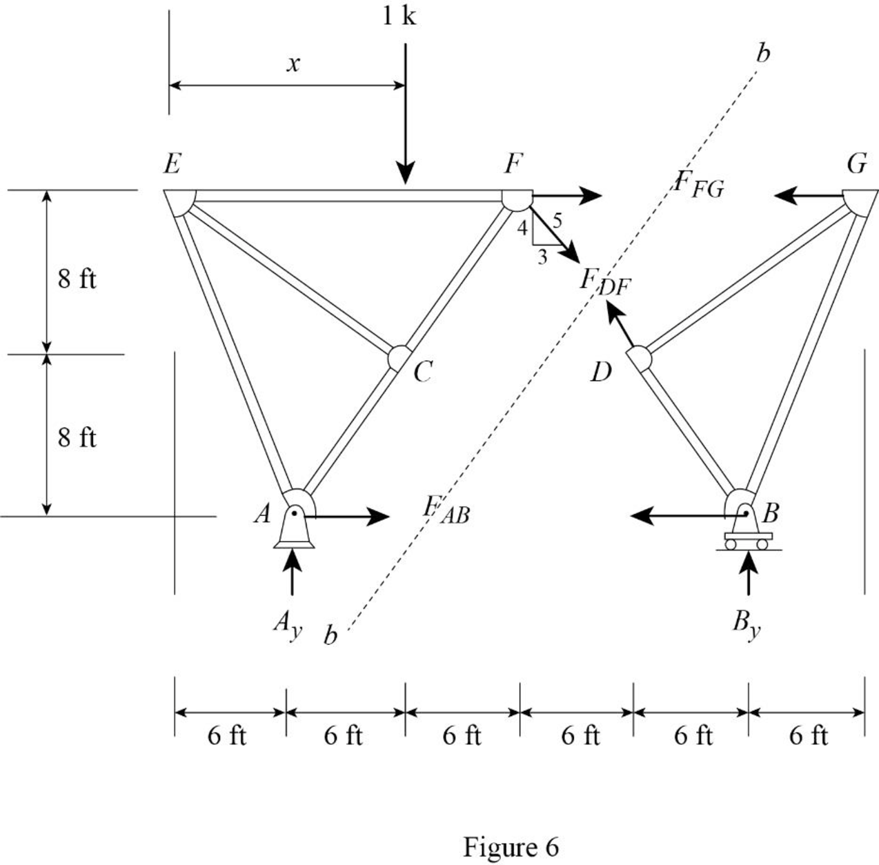
Refer Figure 6.
Find the force in member DF.
Apply 1 k load just left of F
Consider the section right of line bb.
Apply moment equilibrium at G.
Consider clockwise moment as positive and anticlockwise moment as negative.
Substitute
Apply 1 k load just right of F
Consider the section left of line bb.
Apply moment equilibrium at E.
Consider clockwise moment as positive and anticlockwise moment as negative.
Substitute
Thus, the equation of force in the member DF,
Find the force in member DF using the Equation (5) and (6) and then summarize the value in Table 3.
| x (ft) | Apply 1 k load | Force in member DF (k) | Influence line ordinate for the force in member DF (k/k) |
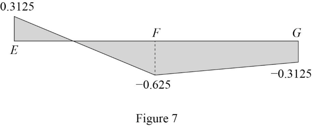
| 0 | E | 0.3125 | |
| 18 | F | ‑0.625 | ‑0.625 |
| 36 | G | ‑0.3125 | ‑0.3125 |
Sketch the influence line diagram for ordinate for the force in member DF using Table 3 as shown in Figure 7.
Influence line for the force in member FG.
Refer Figure 6.
Find the force in member FG.
Apply 1 k load just left of F
Consider the section right of line bb.
Apply moment equilibrium at B.
Consider clockwise moment as positive and anticlockwise moment as negative.
Apply 1 k load just right of F
Consider the section left of line bb.
Apply moment equilibrium at A.
Consider clockwise moment as positive and anticlockwise moment as negative.
Substitute
Thus, the equation of force in the member FG,
Find the force in member FG using the Equation (7) and (8) and then summarize the value in Table 4.
| x (ft) | Apply 1 k load | Force in member FG (k) | Influence line ordinate for the force in member FG (k/k) |
| 0 | E | 0.3125 | |
| 18 | F | ‑0.625 | ‑0.625 |
| 36 | G | ‑0.3125 | ‑0.3125 |
Sketch the influence line diagram for ordinate for the force in member FG using Table 4 as shown in Figure 8.
Want to see more full solutions like this?
Chapter 8 Solutions
STRUCTURAL ANALYSIS (LL)


- I need help setti if this problem up and solving. I keep doing something wrong.arrow_forward1.0 m (Eccentricity in one direction only)=0.15 m Call 1.5 m x 1.5m Centerline An eccentrically loaded foundation is shown in the figure above. Use FS of 4 and determine the maximum allowable load that the foundation can carry if y = 18 kN/m³ and ' = 35°. Use Meyerhof's effective area method. For '=35°, N = 33.30 and Ny = 48.03. (Enter your answer to three significant figures.) Qall = kNarrow_forwardWhat are some advantages and disadvantages of using prefabrication in construction to improve efficiency and cut down on delays?arrow_forward
- PROBLEM:7–23. Determine the maximum shear stress acting in the beam at the critical section where the internal shear force is maximum. 3 kip/ft ΑΟ 6 ft DiC 0.75 in. 6 ft 6 in. 1 in. F [ 4 in. C 4 in. D 6 in. Fig of prob:7-23 1 in. 6 ft Barrow_forward7.60 This abrupt expansion is to be used to dissipate the high-energy flow of water in the 5-ft-diameter penstock. Assume α = 1.0 at all locations. a. What power (in horsepower) is lost through the expansion? b. If the pressure at section 1 is 5 psig, what is the pressure at section 2? c. What force is needed to hold the expansion in place? 5 ft V = 25 ft/s Problem 7.60 (2) 10 ftarrow_forward7.69 Assume that the head loss in the pipe is given by h₁ = 0.014(L/D) (V²/2g), where L is the length of pipe and D is the pipe diameter. Assume α = 1.0 at all locations. a. Determine the discharge of water through this system. b. Draw the HGL and the EGL for the system. c. Locate the point of maximum pressure. d. Locate the point of minimum pressure. e. Calculate the maximum and minimum pressures in the system. Elevation 100 m Water T = 10°C L = 100 m D = 60 cm Elevation 95 m Elevation 100 m L = 400 m D = 60 cm Elevation = 30 m Nozzle 30 cm diameter jet Problem 7.69arrow_forward
- A rectangular flume of planed timber (n=0.012) slopes 0.5 ft per 1000 ft. (i)Compute the discharge if the width is 7 ft and the depth of water is 3.5 ft. (ii) What would be thedischarge if the width were 3.5 ft and depth of water is 7 ft? (iii) Which of the two forms wouldhave greater capacity and which would require less lumber?arrow_forwardFigure shows a tunnel section on the Colorado River Aqueduct. The area of the water cross section is 191 ft 2 , and the wetted perimeter is 39.1 ft. The flow is 1600 cfs. If n=0.013 for the concrete lining, find the slope.arrow_forward7.48 An engineer is making an estimate for a home owner. This owner has a small stream (Q= 1.4 cfs, T = 40°F) that is located at an elevation H = 34 ft above the owner's residence. The owner is proposing to dam the stream, diverting the flow through a pipe (penstock). This flow will spin a hydraulic turbine, which in turn will drive a generator to produce electrical power. Estimate the maximum power in kilowatts that can be generated if there is no head loss and both the turbine and generator are 100% efficient. Also, estimate the power if the head loss is 5.5 ft, the turbine is 70% efficient, and the generator is 90% efficient. Penstock Turbine and generator Problem 7.48arrow_forward
- design rectangular sections for the beam and loads, and p values shown. Beam weights are not included in the loads given. Show sketches of cross sections including bar sizes, arrangements, and spacing. Assume concrete weighs 23.5 kN/m'. fy= 420 MPa, and f’c= 21 MPa.Show the shear and moment diagrams as wellarrow_forwardDraw as a 3D object/Isometricarrow_forwardPost-tensioned AASHTO Type II girders are to be used to support a deck with unsupported span equal to 10 meters. Two levels of Grade 250, 10 x 15.2 mm Ø 7-wire strand are used to tension the girders with 5 tendons per level, where the tendons on top stressed before the ones on the bottom. The girder is simply supported at both ends. The anchors are located 100 mm above the neutral axis at the supports while the eccentricity is measured at 400 mm at the midspan. The tendon profile follows a parabolic shape using a rigid metal sheathing. A concrete topping (slab) 130 mm thick is placed above the beam with a total tributary width of 4 meters. Use maximum values for ranges (table values). Assume that the critical section of the beam is at 0.45LDetermine the losses (friction loss, anchorage, elastic shortening, creep, shrinkage, relaxation). Determine the stresses at the top fibers @ critical section before placing a concrete topping, right after stress transfer. Determine the stress at the…arrow_forward