Concept explainers
Videos
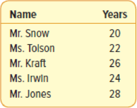
The years of service of the five executives employed by Standard Chemicals are:
- (a) Using the combination formula, how many
samples of size 2 are possible? - (b) List all possible samples of two executives from the population and compute their means.
- (c) Organize the means into a sampling distribution.
- (d) Compare the population
mean and the mean of the sample means. - (e) Compare the dispersion in the population with that in the distribution of the sample mean.
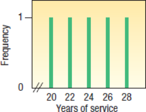
- (f) A chart portraying the population values follows. Is the distribution of population values
normally distributed (bell-shaped)?
- (g) Is the distribution of the sample mean computed in part (c) starting to show some tendency toward being bell-shaped?
a.
Find the possible number of samples of size 2 using combination formula.
Answer to Problem 3SR
The possible number of samples of size 2 using combination formula is 10.
Explanation of Solution
From the given information, the years of service of the five executives are 20, 22, 26, 24 and 28.
The possible number of different samples of size two is obtained by using the following formula:
Substitute 5 for the N and 2 for the n
Then,
Thus, the possible number of samples of size 2 using combination formula is 10.
b.
Give the all possible samples of two executives.
Find the mean of each sample.
Answer to Problem 3SR
Thus, all possible samples of two executives are
Thus, the mean of each sample is 21, 23, 22, 24, 24, 23, 25, 25, 27 and 26.
Explanation of Solution
The mean is calculated by using the following formula:
| Sample | Mean |
Thus, all possible samples of size 2 are
Thus, the mean of each sample is 21, 23, 22, 24, 24, 23, 25, 25, 27 and 26.
c.
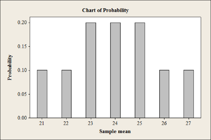
Construct the sampling distribution for the means.
Answer to Problem 3SR
The sampling distribution for the means is
Explanation of Solution
The sampling distribution for the means is as follows:
| Sample mean | Frequency | Probability |
| 21 | 1 | |
| 22 | 1 | |
| 23 | 2 | |
| 24 | 2 | |
| 25 | 2 | |
| 26 | 1 | |
| 27 | 1 | |
Software procedure:
Step-by-step procedure to obtain the bar chart using MINITAB:
- Choose Stat > Graph > Bar chart.
- Under Bars represent, enter select Values from a table.
- Under One column of values select Simple.
- Click on OK.
- Under Graph variables enter probability and under categorical variable enter sample mean.
- Click OK.
Output using MINITAB software is given below:

d.
Give the comparison between the population mean and the mean of the sample means.
Answer to Problem 3SR
The mean of the distribution of the sample means is equal to the population mean.
Explanation of Solution
Population mean is calculated as follows:
The mean of the sample means is calculated as follows:
Comparison:
The mean of the distribution of the sample mean is 24 and the population mean is 24. The two means are exactly same.
Thus, the mean of the distribution of the sample means is equal to the population mean.
e.
Give the dispersion in the population with that in the distribution of the sample mean.
Answer to Problem 3SR
The dispersion in the population is greater than with that of the sample mean.
Explanation of Solution
The population values are 20, 22, 26, 24 and 28. From the part b, the mean of each sample is 21, 23, 22, 24, 24, 23, 25, 25, 27 and 26.
The population values are between 20 and 28. The sample mean values are between 21 and 27.
Thus, the dispersion in the population is greater than with that of the sample mean.
f.
Check whether the distribution of population values is normally distributed or not.
Answer to Problem 3SR
The distribution of population values is not normally distributed.
Explanation of Solution
From the given chart, the frequency of all the years of service is at same level. Then, the distribution of the population values is uniform.
Thus, the distribution of population values is not normally distributed.
g.
Check whether the distribution of the sample mean computed in part (c) starting to show some tendency toward being bell-shaped or not.
Answer to Problem 3SR
The distribution of the sample mean computed in part (c) starting to show some tendency toward being bell-shaped.
Explanation of Solution
From the part (c), it can be observed that the shape of the bar chart is bell shaped.
Thus, the distribution of the sample mean computed in part (c) starting to show some tendency toward being bell-shaped.
Want to see more full solutions like this?
Chapter 8 Solutions
EBK STATISTICAL TECHNIQUES IN BUSINESS


- Question 2 Parts manufactured by an injection molding process are subjected to a compressive strength test. Twenty samples of five parts each are collected, and the compressive strengths (in psi) are shown in Table 2. Table 2: Strength Data for Question 2 Sample Number x1 x2 23 x4 x5 R 1 83.0 2 88.6 78.3 78.8 3 85.7 75.8 84.3 81.2 78.7 75.7 77.0 71.0 84.2 81.0 79.1 7.3 80.2 17.6 75.2 80.4 10.4 4 80.8 74.4 82.5 74.1 75.7 77.5 8.4 5 83.4 78.4 82.6 78.2 78.9 80.3 5.2 File Preview 6 75.3 79.9 87.3 89.7 81.8 82.8 14.5 7 74.5 78.0 80.8 73.4 79.7 77.3 7.4 8 79.2 84.4 81.5 86.0 74.5 81.1 11.4 9 80.5 86.2 76.2 64.1 80.2 81.4 9.9 10 75.7 75.2 71.1 82.1 74.3 75.7 10.9 11 80.0 81.5 78.4 73.8 78.1 78.4 7.7 12 80.6 81.8 79.3 73.8 81.7 79.4 8.0 13 82.7 81.3 79.1 82.0 79.5 80.9 3.6 14 79.2 74.9 78.6 77.7 75.3 77.1 4.3 15 85.5 82.1 82.8 73.4 71.7 79.1 13.8 16 78.8 79.6 80.2 79.1 80.8 79.7 2.0 17 82.1 78.2 18 84.5 76.9 75.5 83.5 81.2 19 79.0 77.8 20 84.5 73.1 78.2 82.1 79.2 81.1 7.6 81.2 84.4 81.6 80.8…arrow_forwardName: Lab Time: Quiz 7 & 8 (Take Home) - due Wednesday, Feb. 26 Contingency Analysis (Ch. 9) In lab 5, part 3, you will create a mosaic plot and conducted a chi-square contingency test to evaluate whether elderly patients who did not stop walking to talk (vs. those who did stop) were more likely to suffer a fall in the next six months. I have tabulated the data below. Answer the questions below. Please show your calculations on this or a separate sheet. Did not stop walking to talk Stopped walking to talk Totals Suffered a fall Did not suffer a fall Totals 12 11 23 2 35 37 14 14 46 60 Quiz 7: 1. (2 pts) Compute the odds of falling for each group. Compute the odds ratio for those who did not stop walking vs. those who did stop walking. Interpret your result verbally.arrow_forwardSolve please and thank you!arrow_forward
- 7. In a 2011 article, M. Radelet and G. Pierce reported a logistic prediction equation for the death penalty verdicts in North Carolina. Let Y denote whether a subject convicted of murder received the death penalty (1=yes), for the defendant's race h (h1, black; h = 2, white), victim's race i (i = 1, black; i = 2, white), and number of additional factors j (j = 0, 1, 2). For the model logit[P(Y = 1)] = a + ß₁₂ + By + B²², they reported = -5.26, D â BD = 0, BD = 0.17, BY = 0, BY = 0.91, B = 0, B = 2.02, B = 3.98. (a) Estimate the probability of receiving the death penalty for the group most likely to receive it. [4 pts] (b) If, instead, parameters used constraints 3D = BY = 35 = 0, report the esti- mates. [3 pts] h (c) If, instead, parameters used constraints Σ₁ = Σ₁ BY = Σ; B = 0, report the estimates. [3 pts] Hint the probabilities, odds and odds ratios do not change with constraints.arrow_forwardSolve please and thank you!arrow_forwardSolve please and thank you!arrow_forward
- Question 1:We want to evaluate the impact on the monetary economy for a company of two types of strategy (competitive strategy, cooperative strategy) adopted by buyers.Competitive strategy: strategy characterized by firm behavior aimed at obtaining concessions from the buyer.Cooperative strategy: a strategy based on a problem-solving negotiating attitude, with a high level of trust and cooperation.A random sample of 17 buyers took part in a negotiation experiment in which 9 buyers adopted the competitive strategy, and the other 8 the cooperative strategy. The savings obtained for each group of buyers are presented in the pdf that i sent: For this problem, we assume that the samples are random and come from two normal populations of unknown but equal variances.According to the theory, the average saving of buyers adopting a competitive strategy will be lower than that of buyers adopting a cooperative strategy.a) Specify the population identifications and the hypotheses H0 and H1…arrow_forwardYou assume that the annual incomes for certain workers are normal with a mean of $28,500 and a standard deviation of $2,400. What’s the chance that a randomly selected employee makes more than $30,000?What’s the chance that 36 randomly selected employees make more than $30,000, on average?arrow_forwardWhat’s the chance that a fair coin comes up heads more than 60 times when you toss it 100 times?arrow_forward
- Suppose that you have a normal population of quiz scores with mean 40 and standard deviation 10. Select a random sample of 40. What’s the chance that the mean of the quiz scores won’t exceed 45?Select one individual from the population. What’s the chance that his/her quiz score won’t exceed 45?arrow_forwardSuppose that you take a sample of 100 from a population that contains 45 percent Democrats. What sample size condition do you need to check here (if any)?What’s the standard error of ^P?Compare the standard errors of ^p n=100 for ,n=1000 , n=10,000, and comment.arrow_forwardSuppose that a class’s test scores have a mean of 80 and standard deviation of 5. You choose 25 students from the class. What’s the chance that the group’s average test score is more than 82?arrow_forward
 Glencoe Algebra 1, Student Edition, 9780079039897...AlgebraISBN:9780079039897Author:CarterPublisher:McGraw Hill
 Big Ideas Math A Bridge To Success Algebra 1: Stu...AlgebraISBN:9781680331141Author:HOUGHTON MIFFLIN HARCOURTPublisher:Houghton Mifflin Harcourt
 Functions and Change: A Modeling Approach to Coll...AlgebraISBN:9781337111348Author:Bruce Crauder, Benny Evans, Alan NoellPublisher:Cengage Learning