Chapter 8, Problem 1.2F

History

Where Did Statistics Begin?

The origins of many disciplines are lost in antiquity, but the roots of statistics can be identified with some certainty. Systematic record keeping began in London in 1532 with weekly data collection on deaths. Later in the same decade, official data collection on baptisms, deaths, and marriages began in France. In 1608, the collection of similar vital statistics began in Sweden. Canada conducted the first official census in 1666.

Of course, statistics is more than the collection of data. If there is a founder of statistics, that person must be someone who worked with the data in clever and systematic ways and who used the data to reach conclusions that were not previously evident. Many experts believe that an Englishman named John Graunt deserves the title of the founder of statistics.

John Graunt was born in London in 1620. As the eldest child in a large family, he took up his father’s business as a draper (a dealer in clothing and dry goods). He spent most of his life as a prominent London citizen, until he lost his house and possessions in the Fire of London in 1666. Eight years later, he died in poverty.

It’s not clear how John Graunt became interested in the weekly records of baptisms and burials—known as bilk of mortality—that had been kept in London since 1563. In the preface of his book Natural and Political Observations on the Bills of Mortality, he noted that others “made little other use of them” and wondered “what benefit the knowledge of the same would bring to the World.” He must have worked on his statistical projects for many years before his book was first published in 1662.^*

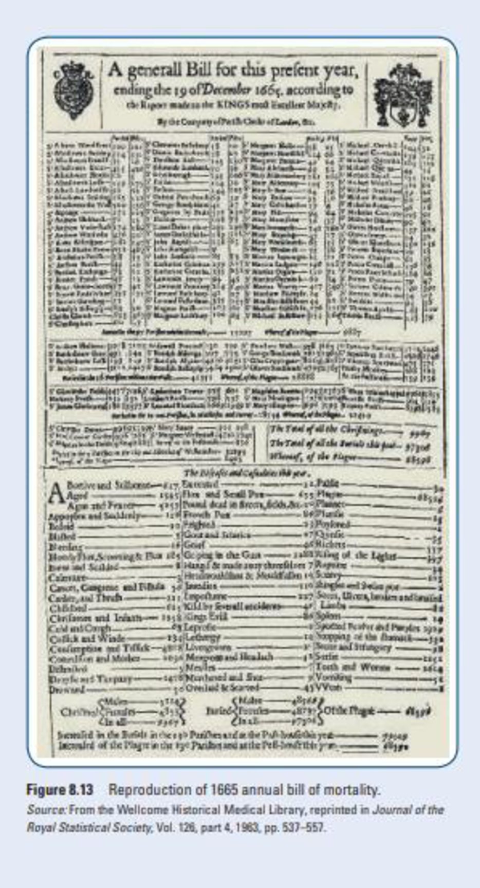
Graunt worked primarily with the annual bills, which were year-end summaries of the weekly bills of mortality. Figure 8.13 shows the annual bill for I66S (the year of the Great Plague). The lop third of the bill shows the numbers of burials and baptisms (christenings) in each parish. Total burials and baptisms arc noted in the middle of the bill, with deaths due to the plague recorded separately. The lower third of the bill shows deaths due to a variety of other causes, with totals given for males and females.

Graunt was aware of rough estimates of the population of London that were made periodically for taxation purposes, but he must have been skeptical of one estimate that put the population of London at 6 or 7 million in 1661. Using the annual bills, comparing burials and baptisms, and estimating the density of families in London (with an average family size of eight), he arrived at a population estimate of 460,000 by three different methods—quite a drop from 6 or 7 million? He also found that the population of London was increasing while the populations of towns in the country side were decreasing, showing an early trend toward urbanization. He raised awareness of the high rates of infant mortality. He also refuted a popular theory that plagues arrive with new kings.

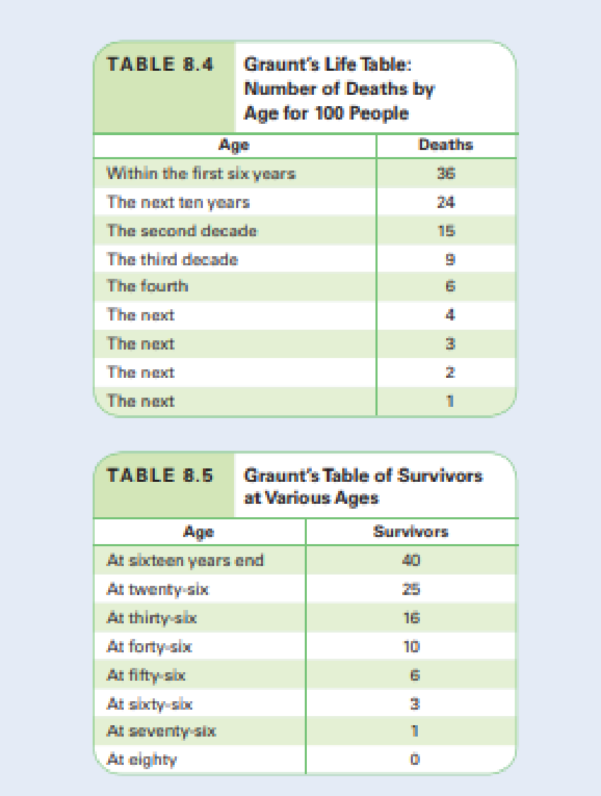
Graunt’s most significant contribution may have been his construction of the first life table. Although detailed data on age at death were not available. Graunt knew that of 100 new babies. “36 of them die before they be six years old. and that perhaps but one survived) 76.” With these two data points, he filled in the intervening years as shown in Table 8.4, using methods that he did not fully explain.

With estimates of deaths for various ages, he was able to make the companion table of survivors shown in Table 8.5. Although some modem statisticians have doubted the methods used to construct these tables. Graunt appears to have appreciated their value and anticipated the actuarial tables now used by life insurance companies. It wasn’t until 1693 that Edmund Halley, of comet fame, constructed life tables using age-based mortality rates.

^*Some historians claim that Graunt’s book was actually written by his lifelong friend and collaborator William Petty, though most statisticians believe Graunt wrote his own book. Either way, we know that Petty continued Graunt’s work, publishing later editions of Graunt’s book and creating the field of “political arithmetic,” which we now call demography.

Do you think that records of burials and baptisms would have given accurate counts of actual births and deaths? Why or why not?