Videos
a.
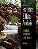
Construct the histogram for body mass of the 50 difference bird species based on the class intervals.
Identify whether transformation of the data is desirable or not.
a.
Answer to Problem 92E
The histogram for body mass of the 50 difference bird species based on the class intervals is given below:
The transformation of the data is desirable.
Explanation of Solution
Calculation:
It is given that the body mass of the 50 different bird species.
Software procedure:
Step-by-step procedure to construct the histogram using the MINITAB software:
- Choose Graph > Histogram.
- Select Simple, and then click OK.
- In Graph variables, enter the corresponding column of Body mass.
- Click OK.
- Double click on x axis and select Binning.
- Choose Cutpoint and enter Number of intervals as 9.
- Enter 5 10 15 20 25 30 40 50 100 500 under Midpoint/Cutpoint positions.
- Click Ok.
From the histogram, it can be observed that most of the data values fall towards the left of the distribution extending the tail towards the right indicating that the distribution of body mass is positively skewed. Thus, for making the data symmetric a transformation is needed.
Hence, the transformation of the data is desirable.
b.
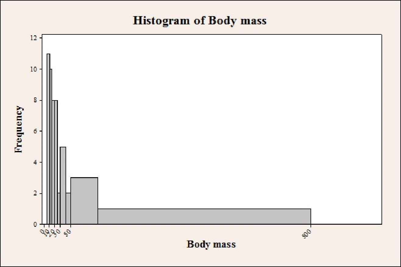
Construct the histogram by transforming the data using logarithms.
Identify whether the log transformation was successful in producing a more symmetric distribution or not.
b.
Answer to Problem 92E
The histogram by transforming the data using logarithms is given below:
Yes, the log transformation was successful in producing a more symmetric distribution.
Explanation of Solution
Calculation:
It is given that the body mass of the 50 different bird species. The log for the data values is obtained as shown below:
| Body Mass | Log (Body Mass) | Transformed values |
| 7.7 | log (7.7) | 0.88649 |
| 10.1 | log (10.1) | 1.00432 |
| 21.6 | log (21.6) | 1.33445 |
| 8.6 | log (8.6) | 0.93450 |
| 12 | log (12) | 1.07918 |
| 11.4 | log (11.4) | 1.05690 |
| 16.6 | log (16.6) | 1.22011 |
| 9.4 | log (9.4) | 0.97313 |
| 11.5 | log (11.5) | 1.06070 |
| 9 | log (9) | 0.95424 |
| 8.2 | log (8.2) | 0.91381 |
| 20.2 | log (20.2) | 1.30535 |
| 48.5 | log (48.5) | 1.68574 |
| 21.6 | log (21.6) | 1.33445 |
| 26.1 | log (26.1) | 1.41664 |
| 6.2 | log (6.2) | 0.79239 |
| 19.1 | log (19.1) | 1.28103 |
| 21 | log (21) | 1.32222 |
| 28.1 | log (28.1) | 1.44871 |
| 10.6 | log (10.6) | 1.02531 |
| 31.6 | log (31.6) | 1.49969 |
| 6.7 | log (6.7) | 0.82607 |
| 5 | log (5) | 0.69897 |
| 68.8 | log (68.8) | 1.83759 |
| 23.9 | log (23.9) | 1.37840 |
| 19.8 | log (19.8) | 1.29667 |
| 20.1 | log (20.1) | 1.30320 |
| 6 | log (6) | 0.77815 |
| 99.6 | log (99.6) | 1.99826 |
| 19.8 | log (19.8) | 1.29667 |
| 16.5 | log (16.5) | 1.21748 |
| 9 | log (9) | 0.95424 |
| 448 | log (448) | 2.65128 |
| 21.3 | log (21.3) | 1.32838 |
| 17.4 | log (17.4) | 1.24055 |
| 36.9 | log (36.9) | 1.56703 |
| 34 | log (34) | 1.53148 |
| 41 | log (41) | 1.61278 |
| 15.9 | log (15.9) | 1.20140 |
| 12.5 | log (12.5) | 1.09691 |
| 10.2 | log (10.2) | 1.00860 |
| 31 | log (31) | 1.49136 |
| 21.5 | log (21.5) | 1.33244 |
| 11.9 | log (11.9) | 1.07555 |
| 32.5 | log (32.5) | 1.51188 |
| 9.8 | log (9.8) | 0.99123 |
| 93.9 | log (93.9) | 0.97267 |
| 10.9 | log (10.9) | 1.03743 |
| 19.6 | log (19.6) | 1.29226 |
| 14.5 | log (14.5) | 1.16137 |
Software procedure:
Step-by-step procedure to obtain histogram using MINITAB:
- Choose Graph > Histogram.
- Choose Simple, and then click OK.
- In Graph variables, enter the corresponding column of Logarithm of Body mass.
- Click OK.
- On graph right click on X axis, select edit X scale.
- Select Binning.
- Under Interval Type, Choose cut point.
- Click OK.
Justification: It can be observed that the histogram of the transformed data (using logarithms) is more near to symmetrical shape when compared to the untransformed data. This shows that using the transformation of logarithms produce a more symmetrical distribution for body mass.
Hence, the log transformation was successful in producing a more symmetric distribution.
c.
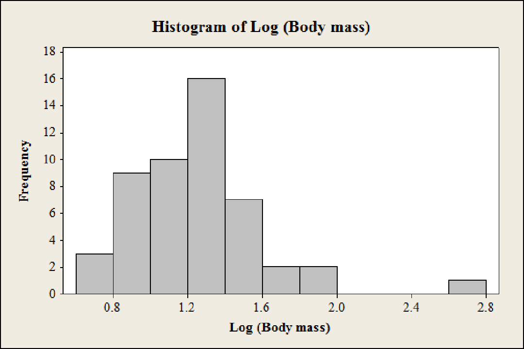
Construct the histogram by transforming the data using
Identify whether the transformation
c.
Answer to Problem 92E
The histogram by transforming the data using
Yes, the transformation
Explanation of Solution
Calculation:
The transformation for the data values using
| Body Mass | Transformed values | |
| 7.7 | 0.360375 | |
| 10.1 | 0.314658 | |
| 21.6 | 0.215166 | |
| 8.6 | 0.340997 | |
| 12 | 0.288675 | |
| 11.4 | 0.296174 | |
| 16.6 | 0.245440 | |
| 9.4 | 0.326164 | |
| 11.5 | 0.294884 | |
| 9 | 0.333333 | |
| 8.2 | 0.349215 | |
| 20.2 | 0.222497 | |
| 48.5 | 0.143592 | |
| 21.6 | 0.215166 | |
| 26.1 | 0.195740 | |
| 6.2 | 0.401610 | |
| 19.1 | 0.228814 | |
| 21 | 0.218218 | |
| 28.1 | 0.188646 | |
| 10.6 | 0.307148 | |
| 31.6 | 0.177892 | |
| 6.7 | 0.386334 | |
| 5 | 0.447214 | |
| 68.8 | 0.120561 | |
| 23.9 | 0.204551 | |
| 19.8 | 0.224733 | |
| 20.1 | 0.223050 | |
| 6 | 0.408248 | |
| 99.6 | 0.100201 | |
| 19.8 | 0.224733 | |
| 16.5 | 0.246183 | |
| 9 | 0.333333 | |
| 448 | 0.017546 | |
| 21.3 | 0.216676 | |
| 17.4 | 0.239732 | |
| 36.9 | 0.164622 | |
| 34 | 0.171499 | |
| 41 | 0.156174 | |
| 15.9 | 0.250785 | |
| 12.5 | 0.282843 | |
| 10.2 | 0.313112 | |
| 31 | 0.179605 | |
| 21.5 | 0.215666 | |
| 11.9 | 0.289886 | |
| 32.5 | 0.175412 | |
| 9.8 | 0.319438 | |
| 93.9 | 0.103197 | |
| 10.9 | 0.302891 | |
| 19.6 | 0.225877 | |
| 14.5 | 0.262613 |
Software procedure:
Step-by-step procedure to obtain histogram using MINITAB:
- Choose Graph > Histogram.
- Choose Simple, and then click OK.
- In Graph variables, enter the corresponding column of 1/sqrt(Body mass).
- Click OK.
- On graph right click on X axis, select edit X scale.
- Select Binning.
- Under Interval Type, Choose cut point.
- Click OK.
Justification: It can be observed that the histogram of the transformed data (using
Hence, the transformation
Want to see more full solutions like this?
Chapter 7 Solutions
Bundle: Introduction to Statistics and Data Analysis, 5th + WebAssign Printed Access Card: Peck/Olsen/Devore. 5th Edition, Single-Term


- Let Y₁, Y2,, Yy be random variables from an Exponential distribution with unknown mean 0. Let Ô be the maximum likelihood estimates for 0. The probability density function of y; is given by P(Yi; 0) = 0, yi≥ 0. The maximum likelihood estimate is given as follows: Select one: = n Σ19 1 Σ19 n-1 Σ19: n² Σ1arrow_forwardPlease could you help me answer parts d and e. Thanksarrow_forwardWhen fitting the model E[Y] = Bo+B1x1,i + B2x2; to a set of n = 25 observations, the following results were obtained using the general linear model notation: and 25 219 10232 551 XTX = 219 10232 3055 133899 133899 6725688, XTY 7361 337051 (XX)-- 0.1132 -0.0044 -0.00008 -0.0044 0.0027 -0.00004 -0.00008 -0.00004 0.00000129, Construct a multiple linear regression model Yin terms of the explanatory variables 1,i, x2,i- a) What is the value of the least squares estimate of the regression coefficient for 1,+? Give your answer correct to 3 decimal places. B1 b) Given that SSR = 5550, and SST=5784. Calculate the value of the MSg correct to 2 decimal places. c) What is the F statistics for this model correct to 2 decimal places?arrow_forward
- Calculate the sample mean and sample variance for the following frequency distribution of heart rates for a sample of American adults. If necessary, round to one more decimal place than the largest number of decimal places given in the data. Heart Rates in Beats per Minute Class Frequency 51-58 5 59-66 8 67-74 9 75-82 7 83-90 8arrow_forwardcan someone solvearrow_forwardQUAT6221wA1 Accessibility Mode Immersiv Q.1.2 Match the definition in column X with the correct term in column Y. Two marks will be awarded for each correct answer. (20) COLUMN X Q.1.2.1 COLUMN Y Condenses sample data into a few summary A. Statistics measures Q.1.2.2 The collection of all possible observations that exist for the random variable under study. B. Descriptive statistics Q.1.2.3 Describes a characteristic of a sample. C. Ordinal-scaled data Q.1.2.4 The actual values or outcomes are recorded on a random variable. D. Inferential statistics 0.1.2.5 Categorical data, where the categories have an implied ranking. E. Data Q.1.2.6 A set of mathematically based tools & techniques that transform raw data into F. Statistical modelling information to support effective decision- making. 45 Q Search 28 # 00 8 LO 1 f F10 Prise 11+arrow_forward
- Students - Term 1 - Def X W QUAT6221wA1.docx X C Chat - Learn with Chegg | Cheg X | + w:/r/sites/TertiaryStudents/_layouts/15/Doc.aspx?sourcedoc=%7B2759DFAB-EA5E-4526-9991-9087A973B894% QUAT6221wA1 Accessibility Mode பg Immer The following table indicates the unit prices (in Rands) and quantities of three consumer products to be held in a supermarket warehouse in Lenasia over the time period from April to July 2025. APRIL 2025 JULY 2025 PRODUCT Unit Price (po) Quantity (q0)) Unit Price (p₁) Quantity (q1) Mineral Water R23.70 403 R25.70 423 H&S Shampoo R77.00 922 R79.40 899 Toilet Paper R106.50 725 R104.70 730 The Independent Institute of Education (Pty) Ltd 2025 Q Search L W f Page 7 of 9arrow_forwardCOM WIth Chegg Cheg x + w:/r/sites/TertiaryStudents/_layouts/15/Doc.aspx?sourcedoc=%7B2759DFAB-EA5E-4526-9991-9087A973B894%. QUAT6221wA1 Accessibility Mode Immersi The following table indicates the unit prices (in Rands) and quantities of three meals sold every year by a small restaurant over the years 2023 and 2025. 2023 2025 MEAL Unit Price (po) Quantity (q0)) Unit Price (P₁) Quantity (q₁) Lasagne R125 1055 R145 1125 Pizza R110 2115 R130 2195 Pasta R95 1950 R120 2250 Q.2.1 Using 2023 as the base year, compute the individual price relatives in 2025 for (10) lasagne and pasta. Interpret each of your answers. 0.2.2 Using 2023 as the base year, compute the Laspeyres price index for all of the meals (8) for 2025. Interpret your answer. Q.2.3 Using 2023 as the base year, compute the Paasche price index for all of the meals (7) for 2025. Interpret your answer. Q Search L O W Larrow_forwardQUAI6221wA1.docx X + int.com/:w:/r/sites/TertiaryStudents/_layouts/15/Doc.aspx?sourcedoc=%7B2759DFAB-EA5E-4526-9991-9087A973B894%7 26 QUAT6221wA1 Q.1.1.8 One advantage of primary data is that: (1) It is low quality (2) It is irrelevant to the purpose at hand (3) It is time-consuming to collect (4) None of the other options Accessibility Mode Immersive R Q.1.1.9 A sample of fifteen apples is selected from an orchard. We would refer to one of these apples as: (2) ھا (1) A parameter (2) A descriptive statistic (3) A statistical model A sampling unit Q.1.1.10 Categorical data, where the categories do not have implied ranking, is referred to as: (2) Search D (2) 1+ PrtSc Insert Delete F8 F10 F11 F12 Backspace 10 ENG USarrow_forward
- epoint.com/:w:/r/sites/TertiaryStudents/_layouts/15/Doc.aspx?sourcedoc=%7B2759DFAB-EA5E-4526-9991-9087A 23;24; 25 R QUAT6221WA1 Accessibility Mode DE 2025 Q.1.1.4 Data obtained from outside an organisation is referred to as: (2) 45 (1) Outside data (2) External data (3) Primary data (4) Secondary data Q.1.1.5 Amongst other disadvantages, which type of data may not be problem-specific and/or may be out of date? W (2) E (1) Ordinal scaled data (2) Ratio scaled data (3) Quantitative, continuous data (4) None of the other options Search F8 F10 PrtSc Insert F11 F12 0 + /1 Backspaarrow_forward/r/sites/TertiaryStudents/_layouts/15/Doc.aspx?sourcedoc=%7B2759DFAB-EA5E-4526-9991-9087A973B894%7D&file=Qu Q.1.1.14 QUAT6221wA1 Accessibility Mode Immersive Reader You are the CFO of a company listed on the Johannesburg Stock Exchange. The annual financial statements published by your company would be viewed by yourself as: (1) External data (2) Internal data (3) Nominal data (4) Secondary data Q.1.1.15 Data relevancy refers to the fact that data selected for analysis must be: (2) Q Search (1) Checked for errors and outliers (2) Obtained online (3) Problem specific (4) Obtained using algorithms U E (2) 100% 高 W ENG A US F10 点 F11 社 F12 PrtSc 11 + Insert Delete Backspacearrow_forwardA client of a commercial rose grower has been keeping records on the shelf-life of a rose. The client sent the following frequency distribution to the grower. Rose Shelf-Life Days of Shelf-Life Frequency fi 1-5 2 6-10 4 11-15 7 16-20 6 21-25 26-30 5 2 Step 2 of 2: Calculate the population standard deviation for the shelf-life. Round your answer to two decimal places, if necessary.arrow_forward
 Glencoe Algebra 1, Student Edition, 9780079039897...AlgebraISBN:9780079039897Author:CarterPublisher:McGraw Hill
 Holt Mcdougal Larson Pre-algebra: Student Edition...AlgebraISBN:9780547587776Author:HOLT MCDOUGALPublisher:HOLT MCDOUGAL