Probability and Statistics for Engineering and the Sciences

9th Edition

ISBN: 9781305251809

Author: Jay L. Devore

Publisher: Cengage Learning

See similar textbooks

Concept explainers

Correlation

Correlation defines a relationship between two independent variables. It tells the degree to which variables move in relation to each other. When two sets of data are related to each other, there is a correlation between them.

Linear Correlation

A correlation is used to determine the relationships between numerical and categorical variables. In other words, it is an indicator of how things are connected to one another. The correlation analysis is the study of how variables are related.

Regression Analysis

Regression analysis is a statistical method in which it estimates the relationship between a dependent variable and one or more independent variable. In simple terms dependent variable is called as outcome variable and independent variable is called as p…

Videos

Textbook Question

Chapter 7.2, Problem 18E

The U.S. Army commissioned a study to assess how deeply a bullet penetrates ceramic body armor (“Testing Body Armor Materials for Use by the U.S. Army-Phase III,” 2012). In the standard test, a cylindrical clay model is layered under the armor vest. A projectile is then fired, causing an indentation in the clay. The deepest impression in the clay is measured as an indication of survivability of someone wearing the armor. Here is data from one testing organization under particular experimental conditions; measurements (in mm) were made using a manually controlled digital caliper:

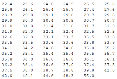
Chapter 7.2, Problem 18E, The U.S. Army commissioned a study to assess how deeply a bullet penetrates ceramic body armor

a. Construct a boxplot of the data and comment on interesting features.
b. Construct a normal probability plot. Is it plausible that impression depth is normally distributed? Is a normal distribution assumption needed in order to calculate a confidence interval or bound for the true average depth μ using the foregoing data? Explain. Use the accompanying Minitab output as a basis for calculating and interpreting an upper confidence bound for μ with a confidence level of 99%.

Variable	Count	Mean	SE Mean	StDev
Depth	83	33.370	0.578	5.268

Q1	Median	Q3	IQR
30.400	33.500	36.000	5.600

Features Features Normal distribution is characterized by two parameters, mean (µ) and standard deviation (σ). When graphed, the mean represents the center of the bell curve and the graph is perfectly symmetric about the center. The mean, median, and mode are all equal for a normal distribution. The standard deviation measures the data's spread from the center. The higher the standard deviation, the more the data is spread out and the flatter the bell curve looks. Variance is another commonly used measure of the spread of the distribution and is equal to the square of the standard deviation.

Expert Solution & Answer

Trending nowThis is a popular solution!

See solution

Check out sample textbook solution

Chapter 7.2, Problem 17E

Chapter 7.2, Problem 19E

Students have asked these similar questions

2.2, 13.2-13.3) question: 5 point(s) possible ubmit test The accompanying table contains the data for the amounts (in oz) in cans of a certain soda. The cans are labeled to indicate that the contents are 20 oz of soda. Use the sign test and 0.05 significance level to test the claim that cans of this soda are filled so that the median amount is 20 oz. If the median is not 20 oz, are consumers being cheated? Click the icon to view the data. What are the null and alternative hypotheses? OA. Ho: Medi More Info H₁: Medi OC. Ho: Medi H₁: Medi Volume (in ounces) 20.3 20.1 20.4 Find the test stat 20.1 20.5 20.1 20.1 19.9 20.1 Test statistic = 20.2 20.3 20.3 20.1 20.4 20.5 Find the P-value 19.7 20.2 20.4 20.1 20.2 20.2 P-value= (R 19.9 20.1 20.5 20.4 20.1 20.4 Determine the p 20.1 20.3 20.4 20.2 20.3 20.4 Since the P-valu 19.9 20.2 19.9 Print Done 20 oz 20 oz 20 oz 20 oz ce that the consumers are being cheated.

T Teenage obesity (O), and weekly fast-food meals (F), among some selected Mississippi teenagers are: Name Obesity (lbs) # of Fast-foods per week Josh 185 10 Karl 172 8 Terry 168 9 Kamie Andy 204 154 12 6 (a) Compute the variance of Obesity, s²o, and the variance of fast-food meals, s², of this data. [Must show full work]. (b) Compute the Correlation Coefficient between O and F. [Must show full work]. (c) Find the Coefficient of Determination between O and F. [Must show full work]. (d) Obtain the Regression equation of this data. [Must show full work]. (e) Interpret your answers in (b), (c), and (d). (Full explanations required). Edit View Insert Format Tools Table

The average miles per gallon for a sample of 40 cars of model SX last year was 32.1, with a population standard deviation of 3.8. A sample of 40 cars from this year’s model SX has an average of 35.2 mpg, with a population standard deviation of 5.4. Find a 99 percent confidence interval for the difference in average mpg for this car brand (this year’s model minus last year’s).Find a 99 percent confidence interval for the difference in average mpg for last year’s model minus this year’s. What does the negative difference mean?

Chapter 7 Solutions

Probability and Statistics for Engineering and the Sciences

Ch. 7.1 - Consider a normal population distribution with the...Ch. 7.1 - Each of the following is a confidence interval for...Ch. 7.1 - Suppose that a random sample of 50 bottles of a...Ch. 7.1 - A CI is desired for the true average stray-load...Ch. 7.1 - Assume that the helium porosity (in percentage) of...Ch. 7.1 - On the basis of extensive tests, the yield point...Ch. 7.1 - By how much must the sample size n be increased if...Ch. 7.1 - Let 1 0, 2 0, with 1 + 2 = . Then P(z1X-/nz2)=1-...Ch. 7.1 - a. Under the same conditions as those leading to...Ch. 7.1 - A random sample of n = 15 heat pumps of a certain...

Ch. 7.1 - Consider the next 1000 95% CIs for that a...Ch. 7.2 - The following observations are lifetimes (days)...Ch. 7.2 - The article Gas Cooking. Kitchen Ventilation, and...Ch. 7.2 - The negative effects of ambient air pollution on...Ch. 7.2 - Determine the confidence level for each of the...Ch. 7.2 - The alternating current (AC) breakdown voltage of...Ch. 7.2 - Exercise 1.13 gave a sample of ultimate tensile...Ch. 7.2 - The U.S. Army commissioned a study to assess how...Ch. 7.2 - The article Limited Yield Estimation for Visual...Ch. 7.2 - TV advertising agencies face increasing challenges...Ch. 7.2 - In a sample of 1000 randomly selected consumers...Ch. 7.2 - The technology underlying hip replacements has...Ch. 7.2 - The Pew Forum on Religion and Public Life reported...Ch. 7.2 - A sample of 56 research cotton samples resulted in...Ch. 7.2 - The Pew Forum on Religion and Public Life reported...Ch. 7.2 - The superintendent of a large school district,...Ch. 7.2 - Reconsider the CI (7.10) for p, and focus on a...Ch. 7.3 - Determine the values of the following quantities:...Ch. 7.3 - Determine the t critical value(s) that will...Ch. 7.3 - Determine the t critical value for a two-sided...Ch. 7.3 - Determine the t critical value for a lower or an...Ch. 7.3 - According to the article Fatigue Testing of...Ch. 7.3 - The article Measuring and Understanding the Aging...Ch. 7.3 - A sample of 14 joint specimens of a particular...Ch. 7.3 - Silicone implant augmentation rhinoplasty is used...Ch. 7.3 - A normal probability plot of the n = 26...Ch. 7.3 - A study of the ability of individuals to walk in a...Ch. 7.3 - Ultra high performance concrete (UHPC) is a...Ch. 7.3 - Exercise 72 of Chapter 1 gave the following...Ch. 7.3 - Prob. 40E Ch. 7.3 - A more extensive tabulation of t critical values...Ch. 7.4 - Determine the values of the following quantities:...Ch. 7.4 - Determine the following: a. The 95th percentile of...Ch. 7.4 - The amount of lateral expansion (mils) was...Ch. 7.4 - Wire electrical-discharge machining (WEDM) is a...Ch. 7.4 - Wire electrical-discharge machining (WEDM) is a...Ch. 7 - Example 1.11 introduced the accompanying...Ch. 7 - The article Distributions of Compressive Strength...Ch. 7 - For those of you who dont already know, dragon...Ch. 7 - A journal article reports that a sample of size 5...Ch. 7 - Unexplained respiratory symptoms reported by...Ch. 7 - High concentration of the toxic element arsenic is...Ch. 7 - Aphid infestation of fruit trees can be controlled...Ch. 7 - It is important that face masks used by...Ch. 7 - A manufacturer of college textbooks is interested...Ch. 7 - The accompanying data on crack initiation depth...Ch. 7 - In Example 6.8, we introduced the concept of a...Ch. 7 - Prob. 58SE Ch. 7 - Prob. 59SE Ch. 7 - Prob. 60SE Ch. 7 - Prob. 61SE Ch. 7 - Prob. 62SE

Knowledge Booster

$Statistics$

Learn more about

Need a deep-dive on the concept behind this application? Look no further. Learn more about this topic, statistics and related others by exploring similar questions and additional content below.

Solution Summary: The author explains how the normal approximation is not mandatory to construct confidence interval about mean.

Concept explainers

Videos

Chapter 7 Solutions