
Concept explainers
Videos
(a)
Section 1:
To find: The difference between the TBBMC recorded for Operator 1 and the TBBMC for Operator 2.
(a)
Section 1:
Answer to Problem 43E
Solution: The table for difference is as follows:
Operator 1 |
Operator 2 |
Difference |
1.328 |
1.323 |
0.005 |
1.342 |
1.322 |
0.02 |
1.075 |
1.073 |
0.002 |
1.228 |
1.233 |
−0.005 |
0.939 |
0.934 |
0.005 |
1.004 |
1.019 |
−0.015 |
1.178 |
1.184 |
−0.006 |
1.286 |
1.304 |
−0.018 |
Explanation of Solution
Calculation:
To calculate the difference, follow the below mentioned steps in Minitab:
Step 1: Enter the variable name as “Operator 1” in column C1 and enter the data for “Operator 1” and enter the variable name as “Operator 2” in column C2 and enter the data for “Operator 2.”
Step 2: Enter variable name as “Difference” in column C3.
Step 3: Go to
Step 4: In the dialog box that appears, select “Difference” in “Store result in variable.”
Step 5: Enter “Operator 1”-“Operator 2” in “Expression.” Click on “Ok” on the dialog box.
From Minitab result, the table for difference is as follows:
Operator 1 |
Operator 2 |
Difference |
1.328 |
1.323 |
0.005 |
1.342 |
1.322 |
0.02 |
1.075 |
1.073 |
0.002 |
1.228 |
1.233 |
−0.005 |
0.939 |
0.934 |
0.005 |
1.004 |
1.019 |
−0.015 |
1.178 |
1.184 |
−0.006 |
1.286 |
1.304 |
−0.018 |
Interpretation: It is clear from the table that the
Section 2:
To test: Whether t- methods can be used or not.
Section 2:
Answer to Problem 43E
Solution: The t- method can be used.
Explanation of Solution
Calculation:
To determine if the t methods can be used or not, a probability plot is drawn in Minitab by following the below mentioned steps:
Step 1: Follow steps 1 and 2 similar to that in Section 1.
Step 2: Go to “Graph” option and click on “Probability Plot.” In the dialog box that appears, select “Single” and click on OK.
Step 3: Then enter the name of the column containing the data of the differences in the “Graph variables” field and click on OK.
The following probability plot is obtained:
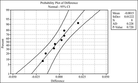
Conclusion: The probability plot shows that the data is approximately normal as all the data points fall within the range and, hence, it is appropriate to use t procedures.
(b)
To test: The significance of the difference between the means of two operators.
(b)
Answer to Problem 43E
Solution: The test statistic value is
Explanation of Solution
Calculation:
To test the null hypothesis, follow the below mentioned steps in Minitab:
Step 1: Follow the Steps 1 to 5 performed in section 1 of part (a).
Step 2: Go to
Step 3: In the dialogue box that appears, select samples in columns.
Step 4: Enter “Operator 1” under the field marked as “First sample” and “Operator 2” under the field marked as “Second sample.”
Step 5: In the dialogue box that appears, Click on “Option.” Enter 95.0 in the field of Confidence interval, 0.0 in “Test mean,” and “not equal” in “Alternative.”
From Minitab results, the value of test statistic is
D.F = n –.
D.F = 8 –.
D.F =.
Conclusion: If the level of significance is 5% then as the p- value is greater than 0.05 the null hypothesis will not be rejected and it is concluded that the two means do not differ significantly at 95% confidence level.
(c)
To find: The confidence interval for difference.
(c)
Answer to Problem 43E
Solution: The required confidence interval is
Explanation of Solution
Calculation: To compute the confidence interval, follow the below mentioned steps in Minitab:
Step 1: Follow the steps 1 to 5 performed in section 1 of part (a).
Step 2: Go to
Step 3: In the dialogue box that appears, select samples in columns.
Step 4: Enter “Operator 1” under the field marked as “First sample” and “Operator 2” under the field marked as “Second sample.”
Step 5: In the dialogue box that appears, Click on “Option.” Enter 95.0 in the field of Confidence interval, 0.0 in “Test mean,” and “not equal” in “Alternative.”
From the Minitab results, the confidence interval is
Interpretation: The confidence interval denotes that the differences recorded will lie in between −0.01172 and 0.00872 with a possible chance of 5% error.
(d)
The validity of the results if the samples are not random.
(d)
Answer to Problem 43E
Solution: The testing results and the confidence interval may not be valid if the samples are non-random.
Explanation of Solution
Want to see more full solutions like this?
Chapter 7 Solutions
EBK INTRODUCTION TO THE PRACTICE OF STA


- I just need to know why this is wrong below: What is the test statistic W? W=5 (incorrect) and What is the p-value of this test? (p-value < 0.001-- incorrect) Use the Wilcoxon signed rank test to test the hypothesis that the median number of pages in the statistics books in the library from which the sample was taken is 400. A sample of 12 statistics books have the following numbers of pages pages 127 217 486 132 397 297 396 327 292 256 358 272 What is the sum of the negative ranks (W-)? 75 What is the sum of the positive ranks (W+)? 5What type of test is this? two tailedWhat is the test statistic W? 5 These are the critical values for a 1-tailed Wilcoxon Signed Rank test for n=12 Alpha Level 0.001 0.005 0.01 0.025 0.05 0.1 0.2 Critical Value 75 70 68 64 60 56 50 What is the p-value for this test? p-value < 0.001arrow_forwardons 12. A sociologist hypothesizes that the crime rate is higher in areas with higher poverty rate and lower median income. She col- lects data on the crime rate (crimes per 100,000 residents), the poverty rate (in %), and the median income (in $1,000s) from 41 New England cities. A portion of the regression results is shown in the following table. Standard Coefficients error t stat p-value Intercept -301.62 549.71 -0.55 0.5864 Poverty 53.16 14.22 3.74 0.0006 Income 4.95 8.26 0.60 0.5526 a. b. Are the signs as expected on the slope coefficients? Predict the crime rate in an area with a poverty rate of 20% and a median income of $50,000. 3. Using data from 50 workarrow_forward2. The owner of several used-car dealerships believes that the selling price of a used car can best be predicted using the car's age. He uses data on the recent selling price (in $) and age of 20 used sedans to estimate Price = Po + B₁Age + ε. A portion of the regression results is shown in the accompanying table. Standard Coefficients Intercept 21187.94 Error 733.42 t Stat p-value 28.89 1.56E-16 Age -1208.25 128.95 -9.37 2.41E-08 a. What is the estimate for B₁? Interpret this value. b. What is the sample regression equation? C. Predict the selling price of a 5-year-old sedan.arrow_forward
- ian income of $50,000. erty rate of 13. Using data from 50 workers, a researcher estimates Wage = Bo+B,Education + B₂Experience + B3Age+e, where Wage is the hourly wage rate and Education, Experience, and Age are the years of higher education, the years of experience, and the age of the worker, respectively. A portion of the regression results is shown in the following table. ni ogolloo bash 1 Standard Coefficients error t stat p-value Intercept 7.87 4.09 1.93 0.0603 Education 1.44 0.34 4.24 0.0001 Experience 0.45 0.14 3.16 0.0028 Age -0.01 0.08 -0.14 0.8920 a. Interpret the estimated coefficients for Education and Experience. b. Predict the hourly wage rate for a 30-year-old worker with four years of higher education and three years of experience.arrow_forward1. If a firm spends more on advertising, is it likely to increase sales? Data on annual sales (in $100,000s) and advertising expenditures (in $10,000s) were collected for 20 firms in order to estimate the model Sales = Po + B₁Advertising + ε. A portion of the regression results is shown in the accompanying table. Intercept Advertising Standard Coefficients Error t Stat p-value -7.42 1.46 -5.09 7.66E-05 0.42 0.05 8.70 7.26E-08 a. Interpret the estimated slope coefficient. b. What is the sample regression equation? C. Predict the sales for a firm that spends $500,000 annually on advertising.arrow_forwardCan you help me solve problem 38 with steps im stuck.arrow_forward
- How do the samples hold up to the efficiency test? What percentages of the samples pass or fail the test? What would be the likelihood of having the following specific number of efficiency test failures in the next 300 processors tested? 1 failures, 5 failures, 10 failures and 20 failures.arrow_forwardThe battery temperatures are a major concern for us. Can you analyze and describe the sample data? What are the average and median temperatures? How much variability is there in the temperatures? Is there anything that stands out? Our engineers’ assumption is that the temperature data is normally distributed. If that is the case, what would be the likelihood that the Safety Zone temperature will exceed 5.15 degrees? What is the probability that the Safety Zone temperature will be less than 4.65 degrees? What is the actual percentage of samples that exceed 5.25 degrees or are less than 4.75 degrees? Is the manufacturing process producing units with stable Safety Zone temperatures? Can you check if there are any apparent changes in the temperature pattern? Are there any outliers? A closer look at the Z-scores should help you in this regard.arrow_forwardNeed help pleasearrow_forward
- Please conduct a step by step of these statistical tests on separate sheets of Microsoft Excel. If the calculations in Microsoft Excel are incorrect, the null and alternative hypotheses, as well as the conclusions drawn from them, will be meaningless and will not receive any points. 4. One-Way ANOVA: Analyze the customer satisfaction scores across four different product categories to determine if there is a significant difference in means. (Hints: The null can be about maintaining status-quo or no difference among groups) H0 = H1=arrow_forwardPlease conduct a step by step of these statistical tests on separate sheets of Microsoft Excel. If the calculations in Microsoft Excel are incorrect, the null and alternative hypotheses, as well as the conclusions drawn from them, will be meaningless and will not receive any points 2. Two-Sample T-Test: Compare the average sales revenue of two different regions to determine if there is a significant difference. (Hints: The null can be about maintaining status-quo or no difference among groups; if alternative hypothesis is non-directional use the two-tailed p-value from excel file to make a decision about rejecting or not rejecting null) H0 = H1=arrow_forwardPlease conduct a step by step of these statistical tests on separate sheets of Microsoft Excel. If the calculations in Microsoft Excel are incorrect, the null and alternative hypotheses, as well as the conclusions drawn from them, will be meaningless and will not receive any points 3. Paired T-Test: A company implemented a training program to improve employee performance. To evaluate the effectiveness of the program, the company recorded the test scores of 25 employees before and after the training. Determine if the training program is effective in terms of scores of participants before and after the training. (Hints: The null can be about maintaining status-quo or no difference among groups; if alternative hypothesis is non-directional, use the two-tailed p-value from excel file to make a decision about rejecting or not rejecting the null) H0 = H1= Conclusion:arrow_forward
 MATLAB: An Introduction with ApplicationsStatisticsISBN:9781119256830Author:Amos GilatPublisher:John Wiley & Sons Inc
 Probability and Statistics for Engineering and th...StatisticsISBN:9781305251809Author:Jay L. DevorePublisher:Cengage Learning
 Statistics for The Behavioral Sciences (MindTap C...StatisticsISBN:9781305504912Author:Frederick J Gravetter, Larry B. WallnauPublisher:Cengage Learning
 Elementary Statistics: Picturing the World (7th E...StatisticsISBN:9780134683416Author:Ron Larson, Betsy FarberPublisher:PEARSON
 The Basic Practice of StatisticsStatisticsISBN:9781319042578Author:David S. Moore, William I. Notz, Michael A. FlignerPublisher:W. H. Freeman
 Introduction to the Practice of StatisticsStatisticsISBN:9781319013387Author:David S. Moore, George P. McCabe, Bruce A. CraigPublisher:W. H. Freeman