
Concept explainers
Videos
Iris setosa is a beautiful wildflower that is found in such diverse places as Alaska, the Gulf of St. Lawrence, much of North America, and even in English meadows and parks. R. A. Fisher, with his colleague Dr. Edgar Anderson, studied these flowers extensively. Dr. Anderson described how he collected information on irises:
I have studied such irises as I could get to see, in as great detail as possible. measuring iris standard after iris standard and iris fall after iris fall, sitting squat-legged with record book and ruler in mountain meadows, in cypress swamps, on lake beaches, and in English parks. [E. Anderson. "The Irises of the Gaspé Peninsula." Bulletin. American IrisSociety, Vol. 59 pp. 2-5, 1935.]
The data in Table 7-10 were collected by Dr. Anderson and were published by his friend and colleague R. A. Fisher in a paper titled "The Use of Multiple Measurements in Taxonomic Problems" (Annals of Eugenics. part II. pp. 179-188, 1936). To find these data, visit the Carnegie Mellon University Data and Story Library (DASI.) web site. From the DASI. site, look under Biology and select Fisher's Irises Story.
Let x be a random variable representing petal length. Using a TI-84Plus/TI-83Plus/TI-n spire calculator, it was found that the sample
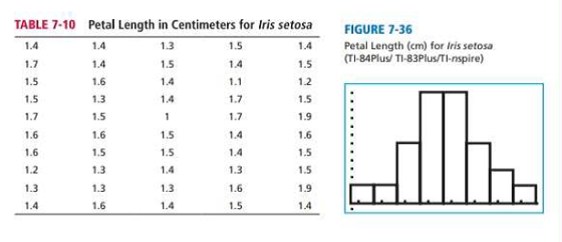
(a) Examine the histogram for petal lengths. Would you say that the distribution is approximately mound-shaped and symmetric? Our sample has only 50 irises; if many thousands of irises had been used, do you think the distribution would look even more like a normal curve? Let x be the petal length of Iris setosa. Research has shown that x has an approximately
(b) Use the
(c) Compute the
(d) Suppose that a random sample of 30 irises is obtained. Compute the probability that the average petal length for this sample is between 1.3 and 1.6 cm. Compute the probability that the average petal length is greater than 1.6 cm.
(e) Compare your answers to parts (c) and (d). Do you notice any differences? Why would these differences occur?
| TABLE 7-10 | Petal Length in Centimeters for Iris serosa | |||
| 1.4 | 14 | 1.3 | 1.5 | 1.4 |
| 1.7 | 1.4 | 1.5 | 14 | 1.5 |
| 1.5 | 1.6 | 14 | 1.1 | 1.2 |
| 1.5 | 1.3 | 1.4 | 1.7 | 1.5 |
| 1.7 | 1.5 | 1 | 1.7 | 1.9 |
| 1.6 | 16 | 1.5 | 1.4 | 16 |
| 1.5 | 1.5 | 1.4 | 1.5 | |
| 1.2 | 1.3 | 1.4 | 1.3 | 1.5 |
| 1.3 | 1.3 | 1.3 | 1.6 | 1.9 |
| 1.4 | 1.6 | 1.4 | 1.5 | 14 |
FIGURE 7-36
Petal Length (cm) for Iris setosa (TI-84Plus/TI-83Plus/TI-n spire)
(a)
To explain: Whether the distribution is approximately mound-shaped and symmetrical.
Answer to Problem DHGP
Solution: Yes, the distribution is approximately mound-shaped and symmetrical.
Explanation of Solution
Calculation:
From the histogram for petal lengths, the distribution is approximately bell-shaped or mound-shaped and symmetrical because approximately the left half of the graph being the mirror image of the right half of the graph.
Our sample has only 50 irises; if many thousands of irises had been used, the distribution would look more similar to normal curve because the sample is very largeand the distribution of the sample will be approximately normally distributed.
(b)
To find: The 68%, 95% and 99% interval and compare the computed percentages with those given by empirical rule..
Answer to Problem DHGP
Solution: The 68%, 95% and 99% interval are (1.3, 1.7), (1.1, 1.9), (0.9, 2.1) respectively.
Explanation of Solution
Let x be the petal length of Iris Setosa and x has an approximately normal distribution, with mean
We know that, 68% of the observations will fall within one standard deviation of mean.
The 68% interval is,
95% of the observations will fall within two standard deviation of mean.
The 95% interval is,
99.7% of the observations will fall within two standard deviation of mean.
The 99.7% interval is,
There are 33 data values fall within the interval 1.3 and 1.7, so the percentage of data within the interval 1.3 and 1.7 is
There are 46 data values fall within the interval 1.1 and 1.9, so the percentage of data within the interval 1.3 and 1.7 is
All data values fall within the interval 0.9 and 2.1, so the percentage of data within the interval 1.3 and 1.7 is
(c)
To find: The probability that a petal length is between 1.3 and 1.6 cm and the probability that a petal length is greater than 1.6 cm.
Answer to Problem DHGP
Solution: The probability that a petal length is between 1.3 and 1.6 cm is 0.5328. The probability that a petal length is greater than 1.6 cm is 0.3085.
Explanation of Solution
Let x be the petal length of Iris Setosa and x has an approximately normal distribution, with mean
We convert the interval
Using Table 3 from the Appendix to find the
Hence, the probability that a petal length is between 1.3 and 1.6 cm is 0.5328.
We convert the interval
Using Table 3 from the Appendix
Hence, the probability that a petal length is greater than 1.6 cm is 0.3085.
(d)
To find: The probability that average petal length is between 1.3 and 1.6 cm and the probability that average petal length is greater than 1.6 cm.
Answer to Problem DHGP
Solution: The probability that average petal length is between 1.3 and 1.6 cm is 0.9972. The probability that averagepetal length is greater than 1.6 cm is 0.0027.
Explanation of Solution
Let x has an approximately normal distribution, with mean
We convert the interval
Using Table 3 from the Appendix
Hence, the probability that average petal length is between 1.3 and 1.6 cm is 0.9972.
We convert the interval
Using Table 3 from the Appendix
Hence, the probability that a petal length is greater than 1.6 cm is 0.0027.
(e)
To explain: The comparison of part (c) and part (d).
Answer to Problem DHGP
Solution:
The standard deviation of the sample mean is much smaller than the population standard deviation.
Explanation of Solution
In part (c), x has a distribution that is approximately normal with
In part (b),
The central limit theorem tells us that the standard deviation of the sample mean is much smaller than the population standard deviation.
Want to see more full solutions like this?
Chapter 7 Solutions
Understanding Basic Statistics


- A marketing agency wants to determine whether different advertising platforms generate significantly different levels of customer engagement. The agency measures the average number of daily clicks on ads for three platforms: Social Media, Search Engines, and Email Campaigns. The agency collects data on daily clicks for each platform over a 10-day period and wants to test whether there is a statistically significant difference in the mean number of daily clicks among these platforms. Conduct ANOVA test. You can provide your answer by inserting a text box and the answer must include: also please provide a step by on getting the answers in excel Null hypothesis, Alternative hypothesis, Show answer (output table/summary table), and Conclusion based on the P value.arrow_forwardA company found that the daily sales revenue of its flagship product follows a normal distribution with a mean of $4500 and a standard deviation of $450. The company defines a "high-sales day" that is, any day with sales exceeding $4800. please provide a step by step on how to get the answers Q: What percentage of days can the company expect to have "high-sales days" or sales greater than $4800? Q: What is the sales revenue threshold for the bottom 10% of days? (please note that 10% refers to the probability/area under bell curve towards the lower tail of bell curve) Provide answers in the yellow cellsarrow_forwardBusiness Discussarrow_forward
- The following data represent total ventilation measured in liters of air per minute per square meter of body area for two independent (and randomly chosen) samples. Analyze these data using the appropriate non-parametric hypothesis testarrow_forwardeach column represents before & after measurements on the same individual. Analyze with the appropriate non-parametric hypothesis test for a paired design.arrow_forwardShould you be confident in applying your regression equation to estimate the heart rate of a python at 35°C? Why or why not?arrow_forward
 Glencoe Algebra 1, Student Edition, 9780079039897...AlgebraISBN:9780079039897Author:CarterPublisher:McGraw Hill
 Holt Mcdougal Larson Pre-algebra: Student Edition...AlgebraISBN:9780547587776Author:HOLT MCDOUGALPublisher:HOLT MCDOUGAL
 Mathematics For Machine TechnologyAdvanced MathISBN:9781337798310Author:Peterson, John.Publisher:Cengage Learning,
 Functions and Change: A Modeling Approach to Coll...AlgebraISBN:9781337111348Author:Bruce Crauder, Benny Evans, Alan NoellPublisher:Cengage Learning