a.
To make: The stem plot for IQ test scores of 31-seventh grade girls.
To check: Whether there are major departures from normality or not.
a.
Answer to Problem 7.59SE
The stem plot is,
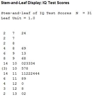
No, there are no major departures from normality.
Explanation of Solution
Given info:
The data shows the IQ test scores of 31 seventh-grade girls in a Midwest school district.
Calculation:
Stemplot:
Software procedure:
Step-by-step software procedure to draw stemplot using MINITAB software is as follows:
- Select Graph > Stem and leaf.
- Select the column of IQ Test Scores in Graph variables.
- Select OK.
The
A observation is a suspected outlier, if it is more than
The difference between the first
That is,
Software procedure:
Step-by-step software procedure for the first quartile and third quartile in MINITAB software is as follows:
- Choose Stat > Basic Statistics > Display
Descriptive Statistics . - In Variables enter the columns IQ Test Scores.
- Choose option statistics, and select first quartile, third quartile.
- Click OK.
Output using MINITAB software is as follows:
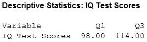
From Minitab output, the first quartile is 98.00 and third quartile is 114.00.
Substitute 114.00 for
The interquartile range is,
Substitute IQR in the
The
Justification:
The stemplot showing that there are two low IQ’s. They are 72 and 74but for the small data, the IQ test scores of 31 seventh-grade girls is approximately normal.
b.
To obtain: The
To check: Whether the proportions show an exactly
b.
Answer to Problem 7.59SE
The mean
The proportions of the scores are within 1 standard deviation of the mean, which is 0.742.
The proportions of the scores are within 2 standard deviation of the mean, which is 0.935.
If the distribution is exactly normal, then its proportion should be about 68% of the observations fall within
Explanation of Solution
If the proportions be in an exactly normal distribution then it is,
About 68% of the observations fall within
About 95% of the observations fall within
About 99.7% of the observations fall within
Calculation:
For Mean and Standard deviation:
Software procedure:
Step-by-step software procedure for mean and standard deviation in MINITAB software is as follows:
- Choose Stat > Basic Statistics > Display Descriptive Statistics.
- In Variables enter the columns IQ Test Scores.
- Choose option statistics, and select mean, standard deviation.
- Click OK.
Output using MINITAB software is as follows:
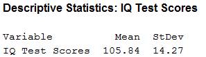
From Minitab output, the mean is 105.84 and standard deviation is 14.27.
The scores are within1 standard deviation and within 2 standard deviations of the mean that are obtained by finding
Substitute 105.84 for x and 14.27 for s,
For proportion of scores within 1 standard deviation:
The IQ test scores in between
The formula to find the proportion of scores within 1 standard deviation is,
Substitute 23 for ‘Number of IQ test scores in between
Thus, the proportion of scores within 1 standard deviation is 0.742.
For proportion of scores within 2 standard deviations:
The IQ test scores in between
The formula to find the proportion of scores within 2 standard deviations is,
Substitute 29 for ‘Number of IQ test scores in between
Thus, the proportion of scores within 2 standard deviations is 0.935.
Justification:
If the distribution is exactly normal, then it should satisfy about 68% of the observations fall within
Here, the proportion of scores within 1 standard deviation is 74.2% and the proportion of scores within 2 standard deviations is 93.5%. Thus, the proportions of scores are reasonably close to the proportion of exactly normal distribution.
Want to see more full solutions like this?
Chapter 7 Solutions
BASIC PRACTICE OF STATS-LL W/SAPLINGPLU

- Suppose the Internal Revenue Service reported that the mean tax refund for the year 2022 was $3401. Assume the standard deviation is $82.5 and that the amounts refunded follow a normal probability distribution. Solve the following three parts? (For the answer to question 14, 15, and 16, start with making a bell curve. Identify on the bell curve where is mean, X, and area(s) to be determined. 1.What percent of the refunds are more than $3,500? 2. What percent of the refunds are more than $3500 but less than $3579? 3. What percent of the refunds are more than $3325 but less than $3579?arrow_forwardA normal distribution has a mean of 50 and a standard deviation of 4. Solve the following three parts? 1. Compute the probability of a value between 44.0 and 55.0. (The question requires finding probability value between 44 and 55. Solve it in 3 steps. In the first step, use the above formula and x = 44, calculate probability value. In the second step repeat the first step with the only difference that x=55. In the third step, subtract the answer of the first part from the answer of the second part.) 2. Compute the probability of a value greater than 55.0. Use the same formula, x=55 and subtract the answer from 1. 3. Compute the probability of a value between 52.0 and 55.0. (The question requires finding probability value between 52 and 55. Solve it in 3 steps. In the first step, use the above formula and x = 52, calculate probability value. In the second step repeat the first step with the only difference that x=55. In the third step, subtract the answer of the first part from the…arrow_forwardIf a uniform distribution is defined over the interval from 6 to 10, then answer the followings: What is the mean of this uniform distribution? Show that the probability of any value between 6 and 10 is equal to 1.0 Find the probability of a value more than 7. Find the probability of a value between 7 and 9. The closing price of Schnur Sporting Goods Inc. common stock is uniformly distributed between $20 and $30 per share. What is the probability that the stock price will be: More than $27? Less than or equal to $24? The April rainfall in Flagstaff, Arizona, follows a uniform distribution between 0.5 and 3.00 inches. What is the mean amount of rainfall for the month? What is the probability of less than an inch of rain for the month? What is the probability of exactly 1.00 inch of rain? What is the probability of more than 1.50 inches of rain for the month? The best way to solve this problem is begin by a step by step creating a chart. Clearly mark the range, identifying the…arrow_forward
- Client 1 Weight before diet (pounds) Weight after diet (pounds) 128 120 2 131 123 3 140 141 4 178 170 5 121 118 6 136 136 7 118 121 8 136 127arrow_forwardClient 1 Weight before diet (pounds) Weight after diet (pounds) 128 120 2 131 123 3 140 141 4 178 170 5 121 118 6 136 136 7 118 121 8 136 127 a) Determine the mean change in patient weight from before to after the diet (after – before). What is the 95% confidence interval of this mean difference?arrow_forwardIn order to find probability, you can use this formula in Microsoft Excel: The best way to understand and solve these problems is by first drawing a bell curve and marking key points such as x, the mean, and the areas of interest. Once marked on the bell curve, figure out what calculations are needed to find the area of interest. =NORM.DIST(x, Mean, Standard Dev., TRUE). When the question mentions “greater than” you may have to subtract your answer from 1. When the question mentions “between (two values)”, you need to do separate calculation for both values and then subtract their results to get the answer. 1. Compute the probability of a value between 44.0 and 55.0. (The question requires finding probability value between 44 and 55. Solve it in 3 steps. In the first step, use the above formula and x = 44, calculate probability value. In the second step repeat the first step with the only difference that x=55. In the third step, subtract the answer of the first part from the…arrow_forward
- If a uniform distribution is defined over the interval from 6 to 10, then answer the followings: What is the mean of this uniform distribution? Show that the probability of any value between 6 and 10 is equal to 1.0 Find the probability of a value more than 7. Find the probability of a value between 7 and 9. The closing price of Schnur Sporting Goods Inc. common stock is uniformly distributed between $20 and $30 per share. What is the probability that the stock price will be: More than $27? Less than or equal to $24? The April rainfall in Flagstaff, Arizona, follows a uniform distribution between 0.5 and 3.00 inches. What is the mean amount of rainfall for the month? What is the probability of less than an inch of rain for the month? What is the probability of exactly 1.00 inch of rain? What is the probability of more than 1.50 inches of rain for the month? The best way to solve this problem is begin by creating a chart. Clearly mark the range, identifying the lower and upper…arrow_forwardProblem 1: The mean hourly pay of an American Airlines flight attendant is normally distributed with a mean of 40 per hour and a standard deviation of 3.00 per hour. What is the probability that the hourly pay of a randomly selected flight attendant is: Between the mean and $45 per hour? More than $45 per hour? Less than $32 per hour? Problem 2: The mean of a normal probability distribution is 400 pounds. The standard deviation is 10 pounds. What is the area between 415 pounds and the mean of 400 pounds? What is the area between the mean and 395 pounds? What is the probability of randomly selecting a value less than 395 pounds? Problem 3: In New York State, the mean salary for high school teachers in 2022 was 81,410 with a standard deviation of 9,500. Only Alaska’s mean salary was higher. Assume New York’s state salaries follow a normal distribution. What percent of New York State high school teachers earn between 70,000 and 75,000? What percent of New York State high school…arrow_forwardPls help asaparrow_forward
- Solve the following LP problem using the Extreme Point Theorem: Subject to: Maximize Z-6+4y 2+y≤8 2x + y ≤10 2,y20 Solve it using the graphical method. Guidelines for preparation for the teacher's questions: Understand the basics of Linear Programming (LP) 1. Know how to formulate an LP model. 2. Be able to identify decision variables, objective functions, and constraints. Be comfortable with graphical solutions 3. Know how to plot feasible regions and find extreme points. 4. Understand how constraints affect the solution space. Understand the Extreme Point Theorem 5. Know why solutions always occur at extreme points. 6. Be able to explain how optimization changes with different constraints. Think about real-world implications 7. Consider how removing or modifying constraints affects the solution. 8. Be prepared to explain why LP problems are used in business, economics, and operations research.arrow_forwardged the variance for group 1) Different groups of male stalk-eyed flies were raised on different diets: a high nutrient corn diet vs. a low nutrient cotton wool diet. Investigators wanted to see if diet quality influenced eye-stalk length. They obtained the following data: d Diet Sample Mean Eye-stalk Length Variance in Eye-stalk d size, n (mm) Length (mm²) Corn (group 1) 21 2.05 0.0558 Cotton (group 2) 24 1.54 0.0812 =205-1.54-05T a) Construct a 95% confidence interval for the difference in mean eye-stalk length between the two diets (e.g., use group 1 - group 2).arrow_forwardAn article in Business Week discussed the large spread between the federal funds rate and the average credit card rate. The table below is a frequency distribution of the credit card rate charged by the top 100 issuers. Credit Card Rates Credit Card Rate Frequency 18% -23% 19 17% -17.9% 16 16% -16.9% 31 15% -15.9% 26 14% -14.9% Copy Data 8 Step 1 of 2: Calculate the average credit card rate charged by the top 100 issuers based on the frequency distribution. Round your answer to two decimal places.arrow_forward
 MATLAB: An Introduction with ApplicationsStatisticsISBN:9781119256830Author:Amos GilatPublisher:John Wiley & Sons Inc
 Probability and Statistics for Engineering and th...StatisticsISBN:9781305251809Author:Jay L. DevorePublisher:Cengage Learning
 Statistics for The Behavioral Sciences (MindTap C...StatisticsISBN:9781305504912Author:Frederick J Gravetter, Larry B. WallnauPublisher:Cengage Learning
 Elementary Statistics: Picturing the World (7th E...StatisticsISBN:9780134683416Author:Ron Larson, Betsy FarberPublisher:PEARSON
 The Basic Practice of StatisticsStatisticsISBN:9781319042578Author:David S. Moore, William I. Notz, Michael A. FlignerPublisher:W. H. Freeman
 Introduction to the Practice of StatisticsStatisticsISBN:9781319013387Author:David S. Moore, George P. McCabe, Bruce A. CraigPublisher:W. H. Freeman