
a.
To construct: The
a.
Answer to Problem 7.40TY
Output using the MINITAB software is given below:
Explanation of Solution
Given info:
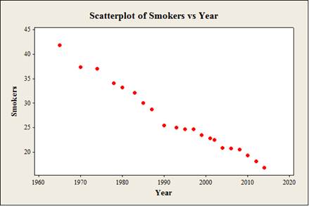
The data shows the year (x) and smokers (y) values.
Calculation:
Step by step procedure to obtain scatterplot using the MINITAB software:
- Choose Graph > Scatterplot.
- Choose Simple and then click OK.
- Under Y variables, enter a column of Smokers.
- Under X variables, enter a column of Year.
- Click OK.
Observation:
From the plot, it is observed that the horizontal axis represents year and vertical axis represents smokers.
b.
To describe: The direction, form, and strength of the relationship between the year and smokers.
To identify: Whether there are any outliers.
b.
Answer to Problem 7.40TY
There is negative direction from the overall pattern.
There is linear form from the overall pattern.
There is a strong relationship between the year and smokers.
There are no outliers from the overall pattern.
Explanation of Solution
Here, the scatterplot is used to describe the direction, form, and strength of the relationship between the year and smokers. Also, the scatterplot is used for identifying the outliers from the overall pattern.
Direction:
The direction shows the overall pattern of the variables. That is, whether the points move from lower left to upper right or from upper left to lower right.
From the scatterplot, it is observed that there is negative direction between the year and smokers because the data points are scattered and move from upper left to lower right.
Form:
The form gives the information about whether the points closely form a straight line, curved or oscillate in some way. That is, it explains about the
From the scatterplot, it is observed that there is linear form between the year and smokers because the data points show the distinct pattern.
Strength:
The strength tells about the overall relationship, that is, whether it is a strong relationship or weak relationship.
Here, from the scatterplot, it is observed that there is a strong relationship between the year and smokers because the data points are closely scattered.
Hence, the relationship was very strong.
Justification:
Outlier:
An observation is said to be an outlier if it is far away from the other observations.
From the scatterplot, it is observed that there is no value which is far away from the other observations. Thus, there is no outlier in the overall pattern.
c.
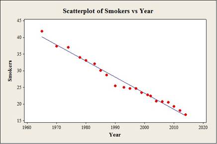
To find: The equation of the least-squares regression line with year (x) as the predictor variable.
To construct: The scatterplot with regression line for the variables year and smokers.
c.
Answer to Problem 7.40TY
The equation of the least-squares regression line with year as the predictor variable (x) is
Output using the MINITAB software is given below:
Explanation of Solution
Calculation:
Regression:
Software procedure:
Step by step procedure to find the equation of the least-squares line by using the MINITAB software:
- Choose Stat > Regression > Regression.
- In Responses, enter the column of Smokers.
- In Predictors, enter the column of Year.
- Click OK.
Output using the MINITAB software is given below:
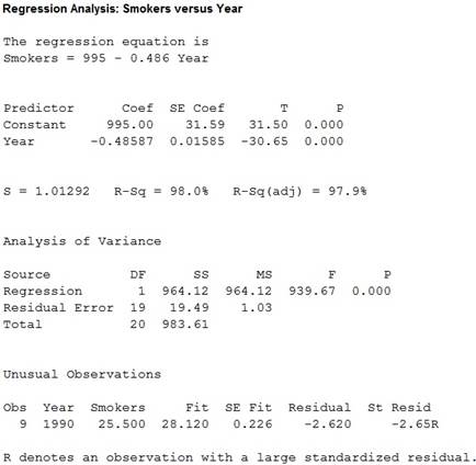
From the MINITAB output, the equation of the least-squares regression line for smokers with year is
Scatterplot:
Step by step procedure to construct the scatterplot using the MINITAB software:
- Choose Graph > Scatterplot.
- Choose With Regression, and then click OK.
- In Responses, enter the column of Smokers.
- In Predictors, enter the column of Year.
- Click OK.
d.
To obtain: Average decrease in smoking per year from 1965 to 2014.
d.
Answer to Problem 7.40TY
The average decrease in smoking per year from 1965 to 2014 is –0.486.
Explanation of Solution
Slope:
It is states the predicted value of y for any given value of x since the response variable (y) is dependent on explanatory variable (x).
Here, the coefficient of x is –0.486. Hence, the slope of the line is negative.
The interpretation for the slope of the line is that, the coefficient value for x is –0.486. Also, the slope indicates for increase in each year, the smokers are decreased by
Thus, the average decrease in smoking per year from 1965 to 2014 is –0.486.
e.
To obtain: The percentage of the observed variation in percent of adults who smoke can be explained by linear change over time.
e.
Answer to Problem 7.40TY
The percentage of the observed variation in percent of adults who smoke can be explained by linear change over time is 98%.
Explanation of Solution
From the MINITAB output for regression in part (c), it is observed that the
Also, the
f.
To find: The predicted the percent of adults who will smoke in 2020.
f.
Answer to Problem 7.40TY
The predicted the percent of adults who will smoke in 2020 is 13.28.
Explanation of Solution
Calculation:
The predicted the percent of adults who will smoke in 2020 is,
Thus, the predicted the percent of adults who will smoke in 2020 is 13.28.
g.
To find: The predicted the percent of adults who will smoke in 2075.
To explain: The reason that the result is impossible.
To explain: The reason that the prediction is made by the regression line to be foolish.
g.
Answer to Problem 7.40TY
The predicted the percent of adults who will smoke in 2075 is –13.45.
The prediction value is impossible because the predicted value of smokers is negative.
The prediction is made by the regression line is foolishness because year 2075 leads to extrapolation.
Explanation of Solution
Calculation:
The predicted the percent of adults who will smoke in 2075 is,
Thus, the predicted the percent of adults who will smoke in 2075 is –13.45. So, the predicted value of smokers is negative.
Hence, the prediction value is impossible.
Justification:
The period of time is from 2014 to 2045. Thus, the year 2075 is far beyond the
Want to see more full solutions like this?
Chapter 7 Solutions
The Basic Practice of Statistics

- Please conduct a step by step of these statistical tests on separate sheets of Microsoft Excel. If the calculations in Microsoft Excel are incorrect, the null and alternative hypotheses, as well as the conclusions drawn from them, will be meaningless and will not receive any points 2. Two-Sample T-Test: Compare the average sales revenue of two different regions to determine if there is a significant difference. (Hints: The null can be about maintaining status-quo or no difference among groups; if alternative hypothesis is non-directional use the two-tailed p-value from excel file to make a decision about rejecting or not rejecting null) H0 = H1=arrow_forwardPlease conduct a step by step of these statistical tests on separate sheets of Microsoft Excel. If the calculations in Microsoft Excel are incorrect, the null and alternative hypotheses, as well as the conclusions drawn from them, will be meaningless and will not receive any points 3. Paired T-Test: A company implemented a training program to improve employee performance. To evaluate the effectiveness of the program, the company recorded the test scores of 25 employees before and after the training. Determine if the training program is effective in terms of scores of participants before and after the training. (Hints: The null can be about maintaining status-quo or no difference among groups; if alternative hypothesis is non-directional, use the two-tailed p-value from excel file to make a decision about rejecting or not rejecting the null) H0 = H1= Conclusion:arrow_forwardPlease conduct a step by step of these statistical tests on separate sheets of Microsoft Excel. If the calculations in Microsoft Excel are incorrect, the null and alternative hypotheses, as well as the conclusions drawn from them, will be meaningless and will not receive any points. The data for the following questions is provided in Microsoft Excel file on 4 separate sheets. Please conduct these statistical tests on separate sheets of Microsoft Excel. If the calculations in Microsoft Excel are incorrect, the null and alternative hypotheses, as well as the conclusions drawn from them, will be meaningless and will not receive any points. 1. One Sample T-Test: Determine whether the average satisfaction rating of customers for a product is significantly different from a hypothetical mean of 75. (Hints: The null can be about maintaining status-quo or no difference; If your alternative hypothesis is non-directional (e.g., μ≠75), you should use the two-tailed p-value from excel file to…arrow_forward
- Please conduct a step by step of these statistical tests on separate sheets of Microsoft Excel. If the calculations in Microsoft Excel are incorrect, the null and alternative hypotheses, as well as the conclusions drawn from them, will be meaningless and will not receive any points. 1. One Sample T-Test: Determine whether the average satisfaction rating of customers for a product is significantly different from a hypothetical mean of 75. (Hints: The null can be about maintaining status-quo or no difference; If your alternative hypothesis is non-directional (e.g., μ≠75), you should use the two-tailed p-value from excel file to make a decision about rejecting or not rejecting null. If alternative is directional (e.g., μ < 75), you should use the lower-tailed p-value. For alternative hypothesis μ > 75, you should use the upper-tailed p-value.) H0 = H1= Conclusion: The p value from one sample t-test is _______. Since the two-tailed p-value is _______ 2. Two-Sample T-Test:…arrow_forwardPlease conduct a step by step of these statistical tests on separate sheets of Microsoft Excel. If the calculations in Microsoft Excel are incorrect, the null and alternative hypotheses, as well as the conclusions drawn from them, will be meaningless and will not receive any points. What is one sample T-test? Give an example of business application of this test? What is Two-Sample T-Test. Give an example of business application of this test? .What is paired T-test. Give an example of business application of this test? What is one way ANOVA test. Give an example of business application of this test? 1. One Sample T-Test: Determine whether the average satisfaction rating of customers for a product is significantly different from a hypothetical mean of 75. (Hints: The null can be about maintaining status-quo or no difference; If your alternative hypothesis is non-directional (e.g., μ≠75), you should use the two-tailed p-value from excel file to make a decision about rejecting or not…arrow_forwardThe data for the following questions is provided in Microsoft Excel file on 4 separate sheets. Please conduct a step by step of these statistical tests on separate sheets of Microsoft Excel. If the calculations in Microsoft Excel are incorrect, the null and alternative hypotheses, as well as the conclusions drawn from them, will be meaningless and will not receive any points. What is one sample T-test? Give an example of business application of this test? What is Two-Sample T-Test. Give an example of business application of this test? .What is paired T-test. Give an example of business application of this test? What is one way ANOVA test. Give an example of business application of this test? 1. One Sample T-Test: Determine whether the average satisfaction rating of customers for a product is significantly different from a hypothetical mean of 75. (Hints: The null can be about maintaining status-quo or no difference; If your alternative hypothesis is non-directional (e.g., μ≠75), you…arrow_forward
- What is one sample T-test? Give an example of business application of this test? What is Two-Sample T-Test. Give an example of business application of this test? .What is paired T-test. Give an example of business application of this test? What is one way ANOVA test. Give an example of business application of this test? 1. One Sample T-Test: Determine whether the average satisfaction rating of customers for a product is significantly different from a hypothetical mean of 75. (Hints: The null can be about maintaining status-quo or no difference; If your alternative hypothesis is non-directional (e.g., μ≠75), you should use the two-tailed p-value from excel file to make a decision about rejecting or not rejecting null. If alternative is directional (e.g., μ < 75), you should use the lower-tailed p-value. For alternative hypothesis μ > 75, you should use the upper-tailed p-value.) H0 = H1= Conclusion: The p value from one sample t-test is _______. Since the two-tailed p-value…arrow_forward4. Dynamic regression (adapted from Q10.4 in Hyndman & Athanasopoulos) This exercise concerns aus_accommodation: the total quarterly takings from accommodation and the room occupancy level for hotels, motels, and guest houses in Australia, between January 1998 and June 2016. Total quarterly takings are in millions of Australian dollars. a. Perform inflation adjustment for Takings (using the CPI column), creating a new column in the tsibble called Adj Takings. b. For each state, fit a dynamic regression model of Adj Takings with seasonal dummy variables, a piecewise linear time trend with one knot at 2008 Q1, and ARIMA errors. c. What model was fitted for the state of Victoria? Does the time series exhibit constant seasonality? d. Check that the residuals of the model in c) look like white noise.arrow_forwardce- 216 Answer the following, using the figures and tables from the age versus bone loss data in 2010 Questions 2 and 12: a. For what ages is it reasonable to use the regression line to predict bone loss? b. Interpret the slope in the context of this wolf X problem. y min ball bas oft c. Using the data from the study, can you say that age causes bone loss? srls to sqota bri vo X 1931s aqsini-Y ST.0 0 Isups Iq nsalst ever tom vam noboslios tsb a ti segood insvla villemari aixs-Yediarrow_forward
- 120 110 110 100 90 80 Total Score Scatterplot of Total Score vs. Putts grit bas 70- 20 25 30 35 40 45 50 Puttsarrow_forward10 15 Answer the following, using the figures and tables from the temperature versus coffee sales data from Questions 1 and 11: a. How many coffees should the manager prepare to make if the temperature is 32°F? b. As the temperature drops, how much more coffee will consumers purchase?ov (Hint: Use the slope.) 21 bru sug c. For what temperature values does the voy marw regression line make the best predictions? al X al 1090391-Yrit,vewolf 30-X Inlog arts bauoxs 268 PART 4 Statistical Studies and the Hunt forarrow_forward18 Using the results from the rainfall versus corn production data in Question 14, answer DOV 15 the following: a. Find and interpret the slope in the con- text of this problem. 79 b. Find the Y-intercept in the context of this problem. alb to sig c. Can the Y-intercept be interpreted here? (.ob or grinisiques xs as 101 gniwollol edt 958 orb sz) asiques sich ed: flow wo PEMAIarrow_forward
 MATLAB: An Introduction with ApplicationsStatisticsISBN:9781119256830Author:Amos GilatPublisher:John Wiley & Sons Inc
 Probability and Statistics for Engineering and th...StatisticsISBN:9781305251809Author:Jay L. DevorePublisher:Cengage Learning
 Statistics for The Behavioral Sciences (MindTap C...StatisticsISBN:9781305504912Author:Frederick J Gravetter, Larry B. WallnauPublisher:Cengage Learning
 Elementary Statistics: Picturing the World (7th E...StatisticsISBN:9780134683416Author:Ron Larson, Betsy FarberPublisher:PEARSON
 The Basic Practice of StatisticsStatisticsISBN:9781319042578Author:David S. Moore, William I. Notz, Michael A. FlignerPublisher:W. H. Freeman
 Introduction to the Practice of StatisticsStatisticsISBN:9781319013387Author:David S. Moore, George P. McCabe, Bruce A. CraigPublisher:W. H. Freeman