
Johnson Filtration. Inc., provides maintenance service for water filtration systems throughout southern Florida. Customers contact Johnson with requests for maintenance service on their water filtration systems. To estimate the service time and the service cost. Johnson’s managers want to predict the repair time necessary for each maintenance request. Hence, repair time in hours is the dependent variable. Repair time is believed to be related to three factors: the number of months since the last maintenance service, the type of repair problem (mechanical or electrical), and the repairperson who performs the repair (Donna Newton or Bob Jones). Data for a sample of 10 service calls are reported in the following table:
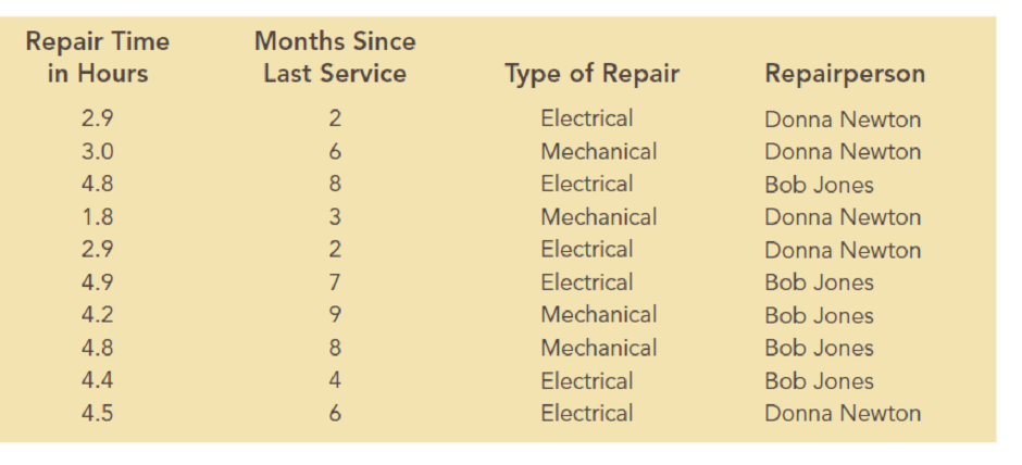
- a. Develop the simple linear regression equation to predict repair time given the number of months since the last maintenance service, and use the results to test the hypothesis that no relationship exists between repair time and the number of months since the last maintenance service at the 0.05 level of significance. What is the interpretation of this relationship? What does the coefficient of determination tell you about this model?
- b. Using the simple linear regression model developed in part (a), calculate the predicted repair time and residual for each of the 10 repairs in the data. Sort the data in ascending order by value of the residual. Do you see any pattern in the residuals for the two types of repair? Do you see any pattern in the residuals for the two repairpersons? Do these results suggest any potential modifications to your simple linear regression model? Now create a scatter chart with months since last service on the x-axis and repair time in hours on the y-axis for which the points representing electrical and mechanical repairs are shown in different shapes and/or colors. Create a similar scatter chart of months since last service and repair time in hours for which the points representing repairs by Bob Jones and Donna Newton are shown in different shapes and/or colors. Do these charts and the results of your residual analysis suggest the same potential modifications to your simple linear regression model?
- c. Create a new dummy variable that is equal to zero if the type of repair is mechanical and one if the type of repair is electrical. Develop the multiple regression equation to predict repair time, given the number of months since the last maintenance service and the type of repair. What are the interpretations of the estimated regression parameters? What does the coefficient of determination tell you about this model?
- d. Create a new dummy variable that is equal to zero if the repairperson is Bob Jones and one if the repairperson is Donna Newton. Develop the multiple regression equation to predict repair time, given the number of months since the last maintenance service and the repairperson. What are the interpretations of the estimated regression parameters? What does the coefficient of determination tell you about this model?
- e. Develop the multiple regression equation to predict repair time, given the number of months since the last maintenance service, the type of repair, and the repairperson. What are the interpretations of the estimated regression parameters? What does the coefficient of determination tell you about this model?
- f. Which of these models would you use? Why?
a.
Find an estimated regression equation that could be used to predict the repair time, given the number of months since the last maintenance service.
Test whether there is any relationship between the repair time and the number of months since the last maintenance service using the level of significance of 0.05. Interpret the test results.
Interpret the value of coefficient of determination.
Answer to Problem 13P
The estimated regression equation that could be used to predict the repair time, given the number of months since the last maintenance service, is
There is sufficient evidence to conclude that there is a linear relationship between the repair time and the number of months since the last maintenance service.
The amount of variation explained in the repair time by the number of months since the last maintenance service is 53.42%.
Explanation of Solution
Calculation:
Here, the repair time is the dependent variable, and the number of months since the last maintenance service is the independent variable.
Step-by-step procedure to obtain the estimated regression equation using EXCEL is defined as follows:
- In EXCEL sheet, enter Repair time in Hours and Months since the last service in columns A and B, respectively.
- In Data, select Data Analysis and choose Regression.
- In Input Y Range, select $A$1:$A$11.
- In Input X Range, select $B$1:$B$11.
- Select Labels.
- Click OK.
Output obtained using EXCEL is given below:
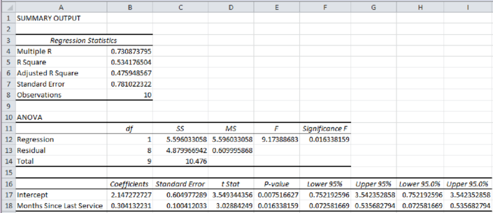
Thus, the estimated regression equation that could be used to predict the repair time, given the number of months since the last maintenance service, is
The null and alternative hypotheses to test whether there is a relationship between repair time and the number of months since the last maintenance service are given as follows:
It is given that the level of significance is 0.05.
From the above output, the P-value is 0.0163.
Decision rule:
The null hypothesis is rejected if the P-value is less than or equal to the level of significance. Otherwise, do not reject the null hypothesis.
Here, the P-value of 0.0163 is less than the level of significance (0.05). Hence, the null hypothesis is rejected.
Therefore, there is sufficient evidence to conclude that there is a linear relationship between the repair time and the number of months since the last maintenance service.
Coefficient of determination:
The coefficient of determination (R-square) value explains the percentage of variation explained in the dependent variable by the independent variables.
From the given output, the value of R-square is approximately 0.5342. That is, the amount of variation explained in the repair time by the number of months since the last maintenance service is 53.42%.
b.
Find the predicted repair time and residual for each of the 10 repairs.
Arrange the data in the ascending order by value of the residual. Is there any pattern observed in the residuals in the two types of repairs. Is there any pattern observed in the residuals in the two repairpersons. Explain whether these results suggest any modifications to the obtained regression model.
Construct a scatterplot with months since the last maintenance service on the x-axis and repair time on the y-axis and differentiate the points between two types of repairs.
Construct a scatterplot with months since the last maintenance service on the x-axis and repair time on the y-axis and differentiate the points between two types of repair persons.
Explain whether these results suggest any modifications to the obtained regression model.
Answer to Problem 13P
The predicted and residual values for all the observations are calculated and given in ascending order by residuals as follows:
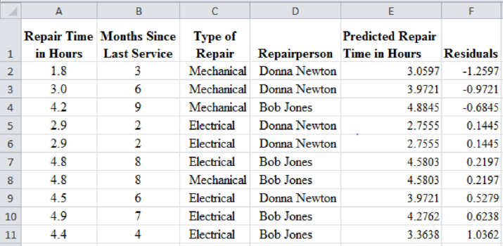
From the above result, mechanical repairs are generally negative residual values and electrical repairs have positive residual values. That is, the mechanical repairs take less time when compared to electrical repairs.
The first two large negative residuals are made by Donna Newton. The residuals of Bob Jones are positive. That is, the repairs by Bob Jones take more time than the predicted values.
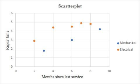
The scatterplots obtained using EXCEL are given below:
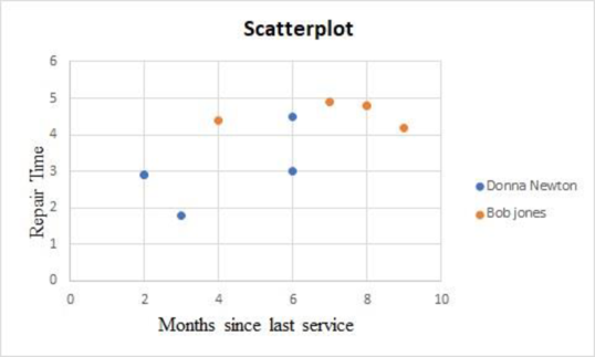
The above results suggest including these categorical variables into the regression model by creating dummy variables.
Explanation of Solution
Calculation:
From the given dataset, the first observation of Months since last service is 2.
The predicted repair time for the first observation is calculated as follows:
Thus, the predicted repair time is 2.7555 hours.
The observed repair time for the first observation is given as 2.9 hours.
The residual of the first observation is calculated as follows:
Similarly, the predicted and residual values for all the observations are calculated and given in the ascending order by residuals as follows:
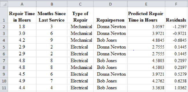
From the above result, mechanical repairs are generally negative residual values and electrical repairs have positive residual values. That is, the mechanical repairs take less time when compared to electrical repairs.
The first two large negative residuals are made by Donna Newton. The residuals of Bob Jones are positive. That is, the repairs by Bob Jones take more time than the predicted values.
The above results suggest including these categorical variables into the regression model by creating dummy variables.
Separate the above data into two tables with respect to the type of repair considering months since last service as follows:
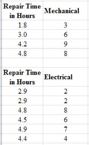
Step-by-step procedure to obtain the scatterplot using EXCEL is given as follows:
- Select the first data with labels.
- Go to Insert, select Charts and select Scatterplot.
- A scatterplot will be displayed.
- Select and copy the second data with labels.
- Click on the scatterplot and click on Paste.
- Select Paste special.
- Select New series and Columns.
- Select Series names in first row and Categories (X values) in first column.
- Click OK.
Output obtained using EXCEL is given below:
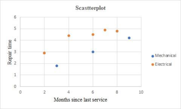
The above chart indicates that the electrical repairs take more time than mechanical repairs.
Separate the above data into two tables with respect to repair person considering months since last service as follows:
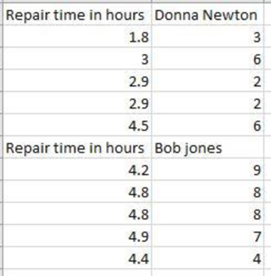
Step-by-step procedure to obtain the scatterplot using EXCEL is given as follows:
- Select the first data with labels.
- Go to Insert, select Charts and select Scatterplot.
- A scatterplot will be displayed.
- Select and copy the second data with labels.
- Click on the scatterplot and click on Paste.
- Select Paste special.
- Select New series and Columns.
- Select Series names in first row and Categories (X values) in first column.
- Click OK.
Output obtained using EXCEL is given below:

The above chart indicates that the repairs by Bob Jones take more time than Donna Newton.
The above two scatterplots suggest including these categorical variables into the regression model by creating dummy variables.
c.
Find an estimated regression equation that could be used to predict the repair time, given the number of months since the last maintenance service and the type of repair.
Interpret the value of coefficient of determination.
Answer to Problem 13P
The estimated regression equation that could be used to predict the repair time, given the number of months since the last maintenance service and the type of repair, is as follows:
It increases every month since the last service will increase the repair time by 0.3876 hours.
The repair time of mechanical repairs is 1.2627 hours less than the repair time of electrical repairs.
The amount of variation explained in the repair time by the number of months since the last maintenance service and the type of repair is 85.92%.
Explanation of Solution
Calculation:
Here, the repair time is the dependent variable. The number of months since the last maintenance service and the type of repair are the independent variables.
Step-by-step procedure to obtain the estimated regression equation using EXCEL is defined as follows:
- Create a variable type of repair.
- In the variable type of repair, enter 0 of the repair is mechanical and enter 1 if the repair is electrical.
- In Data, select Data Analysis and choose Regression.
- In Input Y Range, select $A$1:$A$11.
- In Input X Range, select $B$1:$C$11.
- Select Labels.
- Click OK.
Output obtained using EXCEL is given below:
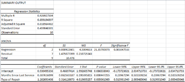
Thus, the estimated regression equation that could be used to predict the repair time, given the number of months since the last maintenance service and the type of repair is as follows:
Interpretation of parameters:
It increases every month since the last service will increase the repair time by 0.3876 hours.
The repair time of mechanical repairs is 1.2627 hours less than the repair time of electrical repairs.
From the given output, the value of R-square is approximately 0.8592. That is, the amount of variation explained in the repair time by the number of months since the last maintenance service and the type of repair is 85.92%.
d.
Find an estimated regression equation that could be used to predict the repair time, given the number of months since the last maintenance service and the repair person.
Interpret the value of coefficient of determination.
Answer to Problem 13P
The estimated regression equation that could be used to predict the repair time, given the number of months since the last maintenance service and the repair person, is as follows:
It increases every month since the last service will increase the repair time by 0.1519 hours.
The repair time of Bob Jones is 1.0835 hours more than the repair time of Donna Newton.
From the given output, the value of R-square is approximately 0.6805. That is, the amount of variation explained in the repair time by the number of months since the last maintenance service and the repairperson is 68.05%.
Explanation of Solution
Calculation:
Here, the repair time is the dependent variable. The number of months since the last maintenance service and the repair person are the independent variables.
Step-by-step procedure to obtain the estimated regression equation using EXCEL is defined as follows:
- Create a variable type of repair.
- In the variable type of repair, enter 0 of the repairperson is Bob Jones and enter 1 if the repairperson is Donna Newton.
- Place the variables repair time, number of months since the last maintenance service, and the repairperson in the columns A, B, and C, respectively.
- In Data, select Data Analysis and choose Regression.
- In Input Y Range, select $A$1:$A$11.
- In Input X Range, select $B$1:$C$11.
- Select Labels.
- Click OK.
Output obtained using EXCEL is given below:
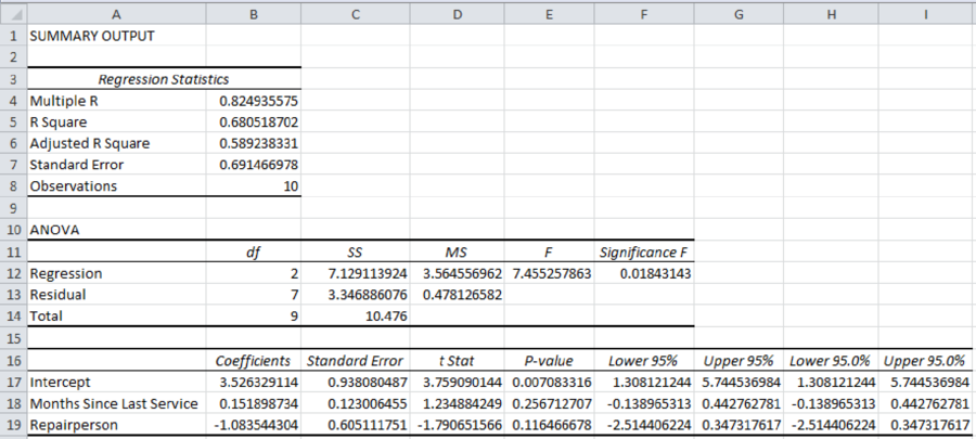
Thus, the estimated regression equation that could be used to predict the repair time, given the number of months since the last maintenance service and the repairperson, is as follows:
Interpretation of parameters:
It increases every month since the last service will increase the repair time by 0.1519 hours.
The repair time of Bob Jones is 1.0835 hours more than the repair time of Donna Newton.
From the given output, the value of R-square is approximately 0.6805. That is, the amount of variation explained in the repair time by the number of months since the last maintenance service and the repairperson is 68.05%.
e.
Find an estimated regression equation that could be used to predict the repair time, given the number of months since the last maintenance service, the type of repair, and the repair person.
Interpret the value of coefficient of determination.
Answer to Problem 13P
The estimated regression equation that could be used to predict the repair time, given the number of months since the last maintenance service, the type of repair, and the repair person is as follows:
It increases every month since the last service will increase the repair time by 0.2914 hours.
The repair time of mechanical repairs is 1.1024 hours less than the repair time of electrical repairs.
The repair time of Bob Jones is 0.6091 hours more than the repair time of Donna Newton.
From the given output, the value of R-square is approximately 0.9002. That is, the amount of variation explained in the repair time by the number of months since the last maintenance service and the repair person is 90.02%.
Explanation of Solution
Calculation:
Here, the repair time is the dependent variable. The number of months since the last maintenance service, the type of repair, and the repairperson are the independent variables.
Step-by-step procedure to obtain the estimated regression equation using EXCEL is defined as follows:
- Place the variables’ repair time, number of months since the last maintenance service, the type of repair, and the repair person in the columns A, B, C, and D, respectively.
- In Data, select Data Analysis and choose Regression.
- In Input Y Range, select $A$1:$A$11.
- In Input X Range, select $B$1:$D$11.
- Select Labels.
- Click OK.
Output obtained using EXCEL is given below:
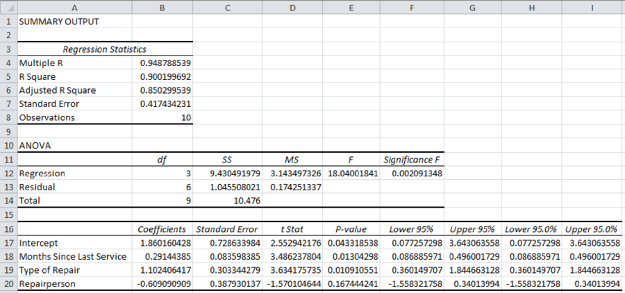
Thus, the estimated regression equation that could be used to predict the repair time, given the number of months since the last maintenance service, the type of repair, and the repair person is as follows:
Interpretation of parameters:
It increases every month since the last service will increase the repair time by 0.2914 hours.
The repair time of mechanical repairs is 1.1024 hours less than the repair time of electrical repairs.
The repair time of Bob Jones is 0.6091 hours more than the repair time of Donna Newton.
From the given output, the value of R-square is approximately 0.9002. That is, the amount of variation explained in the repair time by the number of months since the last maintenance service and the repair person is 90.02%.
f.
Identify the best regression model among the models.
Answer to Problem 13P
The preferable model is the regression model in Part (c).
Explanation of Solution
The R-square value of the regression model in Part (a) is 0.5341. Here, the only independent variable is the number of months since the last maintenance service. Here, the independent variable is significant.
The R-square value of the regression model in Part (c) is 0.8592. Here, the independent variables are the number of months since the last maintenance service and the type of repair. Here, both the independent variables are significant.
The R-square value of the regression model in Part (d) is 0.6805. Here, the independent variables are the number of months since the last maintenance service and the repair person. Here, both the independent variables are insignificant.
The R-square value of the regression model in Part (e) is 0.9002. Here, the independent variables are the number of months since the last maintenance service, the type of repair, and the repair person. Here, the independent variable repair person is insignificant. The value of R-square from the model in Part (c) is increased due to the multicollinearity between the variables such as the number of months since the last maintenance service and the repair person.
The best regression model is always a model with less number of independent variables that are significant and higher value of R-square.
Hence, the preferable model is the regression model in Part (c).
Want to see more full solutions like this?
Chapter 7 Solutions
ESSEN OF BUSINESS ANALYTICS (LL) BOM
- A recent survey of 400 americans asked whether or not parents do too much for their young adult children. The results of the survey are shown in the data file. a) Construct the frequency and relative frequency distributions. How many respondents felt that parents do too much for their adult children? What proportion of respondents felt that parents do too little for their adult children? b) Construct a pie chart. Summarize the findingsarrow_forwardThe average number of minutes Americans commute to work is 27.7 minutes (Sterling's Best Places, April 13, 2012). The average commute time in minutes for 48 cities are as follows: Click on the datafile logo to reference the data. DATA file Albuquerque 23.3 Jacksonville 26.2 Phoenix 28.3 Atlanta 28.3 Kansas City 23.4 Pittsburgh 25.0 Austin 24.6 Las Vegas 28.4 Portland 26.4 Baltimore 32.1 Little Rock 20.1 Providence 23.6 Boston 31.7 Los Angeles 32.2 Richmond 23.4 Charlotte 25.8 Louisville 21.4 Sacramento 25.8 Chicago 38.1 Memphis 23.8 Salt Lake City 20.2 Cincinnati 24.9 Miami 30.7 San Antonio 26.1 Cleveland 26.8 Milwaukee 24.8 San Diego 24.8 Columbus 23.4 Minneapolis 23.6 San Francisco 32.6 Dallas 28.5 Nashville 25.3 San Jose 28.5 Denver 28.1 New Orleans 31.7 Seattle 27.3 Detroit 29.3 New York 43.8 St. Louis 26.8 El Paso 24.4 Oklahoma City 22.0 Tucson 24.0 Fresno 23.0 Orlando 27.1 Tulsa 20.1 Indianapolis 24.8 Philadelphia 34.2 Washington, D.C. 32.8 a. What is the mean commute time for…arrow_forwardMorningstar tracks the total return for a large number of mutual funds. The following table shows the total return and the number of funds for four categories of mutual funds. Click on the datafile logo to reference the data. DATA file Type of Fund Domestic Equity Number of Funds Total Return (%) 9191 4.65 International Equity 2621 18.15 Hybrid 1419 2900 11.36 6.75 Specialty Stock a. Using the number of funds as weights, compute the weighted average total return for these mutual funds. (to 2 decimals) % b. Is there any difficulty associated with using the "number of funds" as the weights in computing the weighted average total return in part (a)? Discuss. What else might be used for weights? The input in the box below will not be graded, but may be reviewed and considered by your instructor. c. Suppose you invested $10,000 in this group of mutual funds and diversified the investment by placing $2000 in Domestic Equity funds, $4000 in International Equity funds, $3000 in Specialty Stock…arrow_forward
- The days to maturity for a sample of five money market funds are shown here. The dollar amounts invested in the funds are provided. Days to Maturity 20 Dollar Value ($ millions) 20 12 30 7 10 5 6 15 10 Use the weighted mean to determine the mean number of days to maturity for dollars invested in these five money market funds (to 1 decimal). daysarrow_forwardc. What are the first and third quartiles? First Quartiles (to 1 decimals) Third Quartiles (to 4 decimals) × ☑ Which companies spend the most money on advertising? Business Insider maintains a list of the top-spending companies. In 2014, Procter & Gamble spent more than any other company, a whopping $5 billion. In second place was Comcast, which spent $3.08 billion (Business Insider website, December 2014). The top 12 companies and the amount each spent on advertising in billions of dollars are as follows. Click on the datafile logo to reference the data. DATA file Company Procter & Gamble Comcast Advertising ($billions) $5.00 3.08 2.91 Company American Express General Motors Advertising ($billions) $2.19 2.15 ETET AT&T Ford Verizon L'Oreal 2.56 2.44 2.34 Toyota Fiat Chrysler Walt Disney Company J.P Morgan a. What is the mean amount spent on advertising? (to 2 decimals) 2.55 b. What is the median amount spent on advertising? (to 3 decimals) 2.09 1.97 1.96 1.88arrow_forwardMartinez Auto Supplies has retail stores located in eight cities in California. The price they charge for a particular product in each city are vary because of differing competitive conditions. For instance, the price they charge for a case of a popular brand of motor oil in each city follows. Also shown are the number of cases that Martinez Auto sold last quarter in each city. City Price ($) Sales (cases) Bakersfield 34.99 501 Los Angeles 38.99 1425 Modesto 36.00 294 Oakland 33.59 882 Sacramento 40.99 715 San Diego 38.59 1088 San Francisco 39.59 1644 San Jose 37.99 819 Compute the average sales price per case for this product during the last quarter? Round your answer to two decimal places.arrow_forward
- Consider the following data and corresponding weights. xi Weight(wi) 3.2 6 2.0 3 2.5 2 5.0 8 a. Compute the weighted mean (to 2 decimals). b. Compute the sample mean of the four data values without weighting. Note the difference in the results provided by the two computations (to 3 decimals).arrow_forwardExpert only,if you don't know it don't attempt it, no Artificial intelligence or screen shot it solvingarrow_forwardFor context, the image provided below is a quesion from a Sepetember, 2024 past paper in statistical modelingarrow_forward
- For context, the images attached below (the question and the related figure) is from a january 2024 past paperarrow_forwardFor context, the image attached below is a question from a June 2024 past paper in statisical modelingarrow_forwardFor context, the images attached below are a question from a June, 2024 past paper in statistical modelingarrow_forward
 Glencoe Algebra 1, Student Edition, 9780079039897...AlgebraISBN:9780079039897Author:CarterPublisher:McGraw Hill
 Functions and Change: A Modeling Approach to Coll...AlgebraISBN:9781337111348Author:Bruce Crauder, Benny Evans, Alan NoellPublisher:Cengage Learning
 Holt Mcdougal Larson Pre-algebra: Student Edition...AlgebraISBN:9780547587776Author:HOLT MCDOUGALPublisher:HOLT MCDOUGAL


