Chapter 6.1, Problem 20E

(a)

To determine

Differences, if any, while comparing the probability distributions of X and Y using histogram.

Answer to Problem 20E

Both distributions are skewed to right with most typical number of rooms in owner − occupied units is 6 rooms and most typical number of rooms in renter − occupied units is 4 rooms.

The owner − occupied units have greater spread and neither distribution shows outliers.

Explanation of Solution

Given information:

X : the number of rooms in randomly selected owner − occupied unit

Y : the number of rooms in randomly selected renter − occupied unit

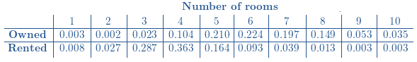
Distributions of the number of rooms for owner − occupied units and renter − occupied units in San Jose, California:

  

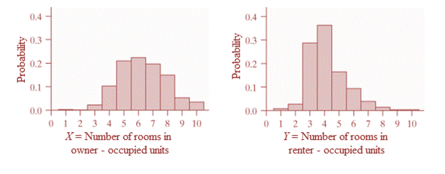
Histograms for X and Y :

  

Shape: In the histograms, the highest bars are slightly to the left, whereas a tail of smaller bars is to the right. Thus, both distributions are slightly skewed to the right.

Center: In first histogram, the highest bar for owner − occupied units is at 6. Thus, the most typical number of rooms in owner − occupied units is 6 rooms.In second histogram, the highest bar for renter − occupied units is at 4. Thus, the most typical number of rooms in renter − occupied units is 4 rooms.

Spread: Since the width of histogram for owner − occupied units is wider than the width of the histogram for renter − occupied units. Thus, the spread of the number of rooms in owner − occupied units is greater than the spread of the number of rooms in renter − occupied units.

Unusual features: Since there are no gaps in the histogram, neither distribution shows outliers.

(b)

To determine

Expected numberof rooms for both types of housing unit and relevance for this difference.

Answer to Problem 20E

Expected number of rooms,

For X :

  ${\mu }_X=6.284\text{rooms}$

For Y :

  ${\mu }_Y=4.187\text{rooms}$

Explanation of Solution

Given information:

X : the number of rooms in randomly selected owner − occupied unit

Y : the number of rooms in randomly selected renter − occupied unit

Distributions of the number of rooms for owner − occupied units and renter − occupied units in San Jose, California:

  

Histograms for X and Y :

  

The expected mean is the sum of the product of each possibility x with its probability $P\left(X=x\right)$ .

For owner - occupied:

  $\begin{array}{l}{\mu }_X={\displaystyle \sum xP\left(X=x\right)}\\ =1\times 0.003+2\times 0.002+3\times 0.023\\ +4\times 0.104+5\times 0.210+6\times 0.224\\ +7\times 0.197+8\times 0.149+9\times 0.053\\ +10\times 0.035\\ =6.284\end{array}$

For rented − occupied:

  $\begin{array}{l}{\mu }_Y={\displaystyle \sum xP\left(X=x\right)}\\ =1\times 0.008+2\times 0.027+3\times 0.287\\ +4\times 0.363+5\times 0.164+6\times 0.093\\ +7\times 0.039+8\times 0.013+9\times 0.003\\ +10\times 0.003\\ =4.187\end{array}$

Now,

Note that

The expected number of rooms for owner − occupied units is greater than the expected number of rooms in renter − occupied units.

Thus,

It makes sense as the peak in the histogram for owner − occupied units is slightly to the right of the peak in the histogram for renter − occupied units.

(c)

To determine

Relevance for the difference in standard deviation of two random variables.

Answer to Problem 20E

The standard deviation confirms the histogram of the owner − occupied units is wider than the histogram of the renter − occupied units.

Explanation of Solution

Given information:

X : the number of rooms in randomly selected owner − occupied unit

Y : the number of rooms in randomly selected renter − occupied unit

Distributions of the number of rooms for owner − occupied units and renter − occupied units in San Jose, California:

  

Histograms for X and Y :

  

Standard deviation of two random variables,

For X :

  ${\sigma }_X=1.640$

For Y :

  ${\sigma }_Y=1.308$

From Part (a),

We conclude that

The spread of the owner - occupied distribution was greater than the spread of the renter - occupied distribution due to wider histogram of the owner − occupied units.

According to the statement,

The standard deviation of “owned” is greater than the standard deviation of “rented”.

Thus,

The standard deviation confirms the conclusion.