
(a)
Interpretation:
Poles and zeros of the given transfer function are to be plotted on a complex plane.
Concept introduction:
For any transfer function
For any transfer function
Answer to Problem 6.1E
The plot of the poles and zeros of the given transfer function on the complex plane as:

Explanation of Solution
Given information:
The given transfer function is:
For the given transfer function, the numerator polynomial is:
To calculate the zeros of the given transfer function, equation this polynomial to zero and calculate its roots using MATLAB commands as shown below:

The compiler will generate its roots as:
These are the zeros of the given transfer function.
For the given transfer function, the denominator polynomial is:
To calculate the poles of the given transfer function, equation this polynomial to zero and calculate its roots using MATLAB commands as shown below:

The compiler will generate its roots as:
These are the poles of the given transfer function.
Now, plot these poles and zeros on the complex plane as:

(b)
Interpretation:
The conclusion regarding the output modes for any input changes is to be determined from the location of poles in the complex plane.
Concept introduction:
For any transfer function
For any transfer function
The complex plane is divided into two halves: Left Half Plane and Right Half Plane. The Left Half Plane represents the stable region and the Right Half Plane represents the unstable region.
Answer to Problem 6.1E
Any change in the input of the process will lead to the unbounded and unstable output as two of the poles of the given transfer function lie in the Right Half Plane.
Explanation of Solution
Given information:
The given transfer function is:
From part (a), the plot of poles and zeros of the given polynomial is:
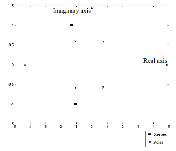
From this plot, two of the poles lie in the Right Half Plane of the complex plane. This makes the process output unstable. Therefore, any change in the input of the process will lead to unbounded and unstable output.
(c)
Interpretation:
The output response for the unit step change in the input for the given transfer function is to be plotted and its correctness to the analysis of the output mode made in part (b) is to be done.
Concept introduction:
For any transfer function
For any transfer function
The complex plane is divided into two halves: Left Half Plane and Right Half Plane. The Left Half Plane represents the stable region and the Right Half Plane represents the unstable region.
Answer to Problem 6.1E
The response of the given transfer function for a unit step change in the input is:
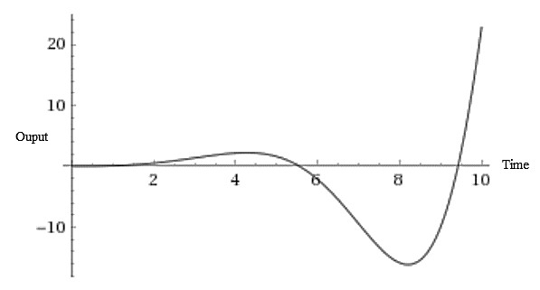
The output response of the process is unstable and unbounded for the step-change in the input which agrees with the analysis done in part (b).
Explanation of Solution
Given information:
The given transfer function is:
For a unit step change in the input, the value of
Substitute this value of
The plot of the response of this transfer function using the online tool will be:

In part (b), it was analyzed that the poles pair in the Right Half Plane makes the system output unbounded and stable. From the response plot shown above, this analysis is correct as the output response of the process is unstable and unbounded for the step-change in the input.
Want to see more full solutions like this?
Chapter 6 Solutions
Process Dynamics And Control, 4e

- A steady Williamson nanofluid containing Cu nanoparticles flows over a permeable wedge with wall suction \( V_w = 0.015 \, \text{m/s} \), under a transverse magnetic field \( B_0 = 0.6 \, \text{T} \). The flow obeys the Buongiorno model, with \( D_B = 9 \times 10^{-10} \), \( D_T = 3.5 \times 10^{-8} \), and activation energy \( E_a = 65 \times 10^3 \). Hall and ion-slip effects are included with \( m_e = 0.4 \), \( \beta = 0.15 \). Thermal conductivity varies as \( k(T) = 0.6 (1 + 0.002 (T - 305)) \). Apply velocity and thermal jump conditions with \( \alpha_u = 0.9 \), \( \alpha_T = 0.8 \), \( \lambda = 2 \times 10^{-7} \). Using Keller’s method and similarity variables for wedge parameter \( m = 0.4 \), determine the entropy generation number \( N_s \) at \( x = 0.03 \), where \[N_s = \frac{k(T)}{T_\infty^2} \left( \frac{\partial T}{\partial y} \right)^2 + \frac{\mu}{T_\infty} \left( \frac{\partial u}{\partial y} \right)^2.\]arrow_forwardE. coli was continuously cultured in a continuous stirred tank fermenter with a working volume of 1 L by chemostat. A medium containing 4.0 g/L of glucose as a carbon source was fed to the fermenter at a constant flow rate of 0.5 L/hr, and the glucose concentration in the output stream was 0.20 g/L. The cell yield with respect to glucose was 0.42 g dry cells per gram glucose.arrow_forwardPlease do not use any AI tools to solve this question. I need a fully manual, step-by-step solution with clear explanations, as if it were done by a human tutor. No AI-generated responses, please.arrow_forward
- In the published paper, "Exergy-based Greenhouse gas metric of buildings", use the value of the Exergy Loss of Emission of carbon dioxide to evaluate the index value for 1000 occupants for 50 years building life span in kilogram per person per yeararrow_forwardA CO₂-saturated brine (ionic strength = 2.5 mol/kg, pH = 3, a_H⁺ = 0.01) flows at 2 cm/s through a horizontal tubular reactor (L = 1 m, D = 0.05 m) packed with 5 kg of olivine (Zhuravlev-BET surface area = 30 m²/g). The system operates at 90 °C and 40 bar, and external mass transfer resistance is negligible. The rate-limiting step is electron transfer at the mineral surface, governed by Marcus theory, with λ = 0.75 eV, ΔG° = –0.30 eV, and k₀ = 10⁶ s⁻¹. The Mg²⁺ activity coefficient is γ = 0.76 (from PHREEQC with Pitzer model). For Mg₂SiO₄ + 4 H⁺ → 2 Mg²⁺ + SiO₂(aq) + 2 H₂O, determine the total moles of Mg²⁺ released after 10 minutes at steady state.arrow_forwardIn baseball, batters frequently attempt to hit a ball as far as possible. However, baseballs are inelastic with an officially required "coefficient of restitution" CR ≈ 0.55 on ash wood. The coefficient of restitution of a dropped ball iswhere H is the initial drop height, h is the max. height on the rebound, and h ≈ 2πH tan δ for a homogeneous material. Assuming that a baseball is homogeneous and has a storage modulus approximately the same as that of cork (E' = 18.6 MPa), what must the value of the loss modulus E'' be so that the ball is regulation?arrow_forward
- The creep strain rate of a polymer (in “Hz”) is given by where T is the temperature and Q = 100. kJ/mol is the activation energy. How long t will it take for a rod of this polymer to extend from 10. mm to 15 mm at 100. °C?arrow_forwardCreep compliance J(t) An amorphous polymer has Tg = 100 °C. A creep modulus of 1/J = 1 GPa was measured after t₁ = 1 h at T₁ = 90 °C. Suppose that log 10 a (T) = 17.5(T-Tg) 52+(T-Tg) 1 for this material. What is the shift factor a at T = T₁ relative to the reference Tg? What is the time t₂ required to reach a modulus of 1 GPa at T2 = 80 °C? TR = T = 100 °C |J(t) = 1 GPa-1 + log a(T₁) T₁ = 75 °C T₂ = 50 °C log tr log t₁ log t log t₂ = ?arrow_forwardA 0.45 mol/kg aqueous solution of 3-(methylamino)propylamine and 1-methylpiperazine (1:1 molar) flows at 0.5 g/s through a 2.5 m horizontal stainless steel coil (inner diameter 1.2 mm), entering at 358.15 K and 22 MPa and exiting at 20 MPa. A constant wall heat flux of 28 W is applied. Local density and isobaric heat capacity are obtained through from the Benedict–Webb–Rubin equation of state, with a 3% increase in heat capacity to account for wall sorption. Dynamic viscosity is obtained using the Green-Kubo relation with a given integral value of 2.1 × 10⁻¹⁰ Pa².s, and thermal conductivity is assumed constant. The local Nusselt number is corrected for thermal development using Nu(x) = 3.66 + (0.065 · Gz(x)^0.7) / (1 + 0.04 · Gz(x)^0.7), where Gz(x) = D · Re(x) · Pr(x) / x. Through a spatially resolved numerical integration of the 1D steady-state energy equation and determine the outlet temperature (K).arrow_forward
- A pilot process is being planned to produce antibiotic P. Antibiotic P is a compound secreted by microorganism A during the stationary phase. To produce P, substrate S is required. The growth of microorganism A follows the Monod equation, with a maximum specific growth rate $\mu_m = 1 h^{-1}$ and a half-saturation constant $K_s = 700\ mg/L$.The pilot process uses a chemostat with a working volume of $1000\ L$. In this chemostat, the outflow is processed to separate microorganisms, which are then concentrated tenfold and recycled. A sterile medium containing $15\ g/L$ of substrate is supplied at a flow rate of $100\ L/h$, while the recycled flow (concentrated) contains $5\ g/L$ and is also fed into the chemostat.Microorganism A yields $0.5\ g$ of biomass per $1\ g$ of substrate consumed $(Y^M_{X/S} = 0.5\ g\ A/g\ S)$, and its death rate $(k_d)$ is negligible. Additionally, $1\ g$ of microorganism A produces $0.05\ g$ of antibiotic P per hour $(q_P = 0.05 g\ P/h\cdot g\ A)$, and $1\ g$…arrow_forwardIn the production of ethyl acetate via reactive distillation, the column operates at 5 bar with an equimolar feed (ethanol + acetic acid) at 80°C. The reaction follows: \[CH_3COOH + C_2H_5OH \rightleftharpoons CH_3COOC_2H_5 + H_2O \quad (K_{eq} = 4.2 \text{ at } 80°C)\] Given: - NRTL parameters for all binary pairs - Tray efficiency = 65% - Vapor-liquid equilibrium exhibits positive azeotrope formation Calculate the exact minimum reflux ratio required to achieve 98% ethyl acetate purity in the distillate, assuming: 1) The reaction reaches equilibrium on each tray 2) The heavy key component is waterarrow_forwardIn a multi-stage distillation column designed to separate a binary mixture of ethanol and water, the mass flow rate of the feed entering the column is \( F \), and the distillate product flow rate is \( D \). The reflux ratio \( R \) is defined as the ratio of the liquid returned to the column to the distillate flow rate. For the ideal case, where the column operates at maximum efficiency, determine the **minimum reflux ratio** \( R_{\text{min}} \) when the relative volatility \( \alpha = 1.5 \).arrow_forward
 Introduction to Chemical Engineering Thermodynami...Chemical EngineeringISBN:9781259696527Author:J.M. Smith Termodinamica en ingenieria quimica, Hendrick C Van Ness, Michael Abbott, Mark SwihartPublisher:McGraw-Hill Education
 Elementary Principles of Chemical Processes, Bind...Chemical EngineeringISBN:9781118431221Author:Richard M. Felder, Ronald W. Rousseau, Lisa G. BullardPublisher:WILEY
 Elements of Chemical Reaction Engineering (5th Ed...Chemical EngineeringISBN:9780133887518Author:H. Scott FoglerPublisher:Prentice Hall
 Industrial Plastics: Theory and ApplicationsChemical EngineeringISBN:9781285061238Author:Lokensgard, ErikPublisher:Delmar Cengage Learning
 Unit Operations of Chemical EngineeringChemical EngineeringISBN:9780072848236Author:Warren McCabe, Julian C. Smith, Peter HarriottPublisher:McGraw-Hill Companies, The