Videos
Since laboratory or field experiments are generally expensive and time consuming,
- a. Use the Osman et al. (2008) method [Eqs. (6.15) through (6.18)].
- b. Use the Gurtug and Sridharan (2004) method [Eqs. (6.13) and (6.14)].
- c. Use the Matteo et al. (2009) method [Eqs. (6.19) and (6.20)].
- d. Plot the calculated wopt against the experimental wopt, and the calculated γd(max) with the experimental γd(max). Draw a 45° line of equality on each plot.
- e. Comment on the predictive capabilities of various methods. What can you say about the inherent nature of empirical models?
(a)
Find the optimum moisture content and maximum dry unit weight using Osman et al. (2008) method.
Explanation of Solution
Calculation:
Determine the plasticity index PI using the relation.
PI=LL−PL
Here, LL is the liquid limit for soil 1 and PL is the plastic limit for soil 1.
Substitute 17 % for LL and 16 % for PL.
PI=17−16=1%
Similarly, calculate the PI for remaining soils.
Determine the optimum moisture content for soil 1 using the relation.
wopt=(1.99−0.165lnE)(PI)
Here, E is the compaction energy for soil 1.
Substitute 2,700 kN-m/m3 for E and 1 % for PI.
wopt=(1.99−0.165ln2,700)(1)=0.69 %
Similarly, calculate the optimum moisture content for remaining soils.
Determine the value of L using the relation.
L=14.34+1.195lnE
Substitute 2,700 kN-m/m3 for E.
L=14.34+1.195ln2,700=23.78
Determine the value of M using the relation.
M=−0.19+0.073lnE
Substitute 2,700 kN-m/m3 for E.
M=−0.19+0.073ln2,700=0.387
Determine the maximum dry unit weight of the soil 1 using the relation.
γd(max)=L−Mwopt
Substitute 23.78 for L, 0.387 for M, and 0.69 % for wopt.
γd(max)=23.78−0.387×0.69=23.51 kN/m3
Similarly, calculate the maximum dry unit weight for remaining soils.
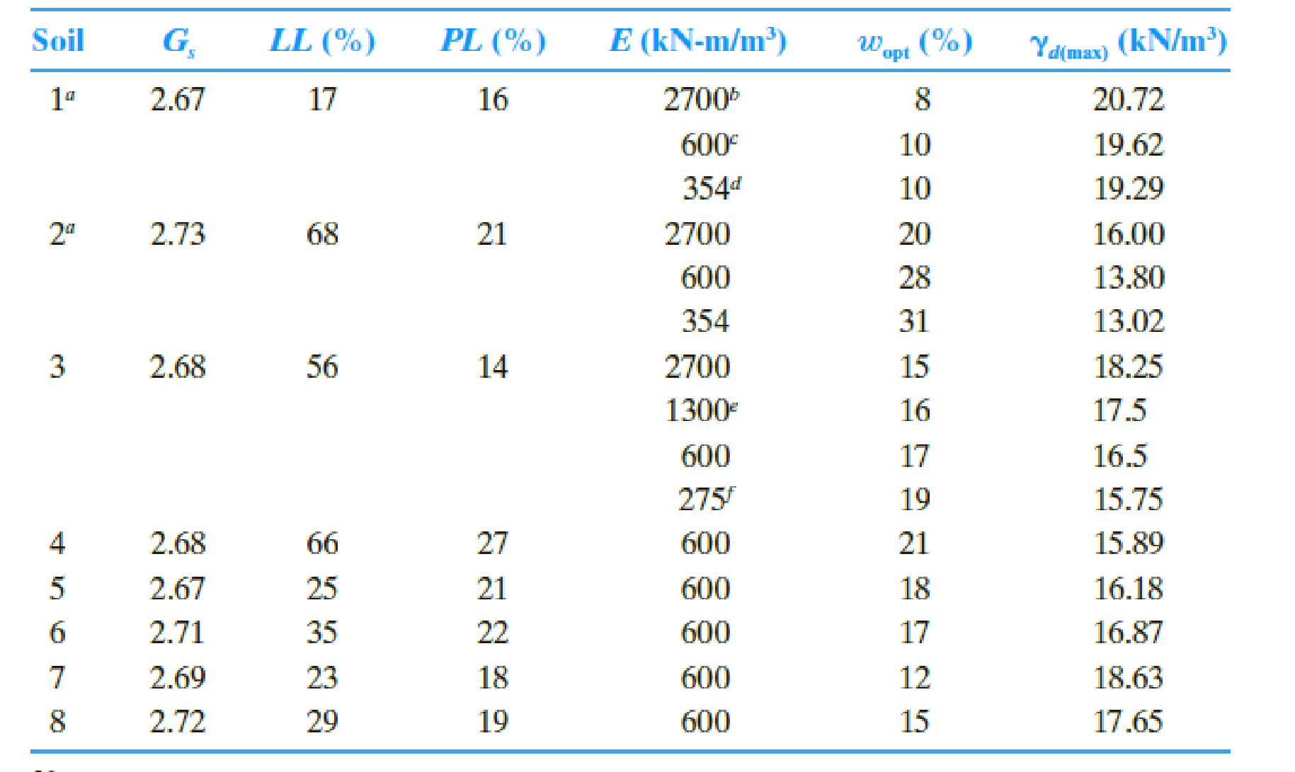
Summarize the calculated values as in Table 1.
| Soil |
LL (%) |
PL (%) |
PI (%) |
E (kN-m/m3) |
wopt(%) (Exp) |
γd(max) (kN/m3) (Exp) |
wopt(%) | L | M |
γd(max)(kN/m3) |
| 1 | 17 | 16 | 1 | 2,700 | 8 | 20.72 | 0.69 | 23.782 | 0.387 | 23.51 |
| 600 | 10 | 19.62 | 0.93 | 21.984 | 0.277 | 21.73 | ||||
| 354 | 10 | 19.29 | 1.02 | 21.354 | 0.238 | 21.11 | ||||
| 2 | 68 | 21 | 47 | 2,700 | 20 | 16.00 | 32.26 | 23.782 | 0.387 | 11.30 |
| 600 | 28 | 13.80 | 43.92 | 21.984 | 0.277 | 9.82 | ||||
| 354 | 31 | 13.02 | 48.01 | 21.354 | 0.238 | 9.91 | ||||
| 3 | 56 | 14 | 42 | 2,700 | 15 | 18.25 | 28.82 | 23.782 | 0.387 | 12.63 |
| 1,300 | 16 | 17.50 | 33.89 | 22.908 | 0.333 | 11.61 | ||||
| 600 | 17 | 16.50 | 39.24 | 21.984 | 0.277 | 11.12 | ||||
| 275 | 19 | 15.75 | 44.65 | 21.052 | 0.220 | 11.23 | ||||
| 4 | 66 | 27 | 39 | 600 | 21 | 15.89 | 36.45 | 21.984 | 0.277 | 11.89 |
| 5 | 25 | 21 | 4 | 600 | 18 | 16.18 | 3.740 | 21.984 | 0.277 | 20.95 |
| 6 | 35 | 22 | 13 | 600 | 17 | 16.87 | 12.15 | 21.984 | 0.277 | 18.62 |
| 7 | 23 | 18 | 5 | 600 | 12 | 18.63 | 4.67 | 21.984 | 0.277 | 20.69 |
| 8 | 29 | 19 | 10 | 600 | 15 | 17.65 | 9.35 | 21.984 | 0.277 | 19.39 |
(b)
Find the optimum moisture content and maximum dry unit weight using Gurtug and Sridharan (2004) method.
Explanation of Solution
Calculation:
Determine the optimum moisture content for soil 1 using the relation.
wopt=(1.95−0.38(logE))(PL)
Substitute 2,700 kN-m/m3 for E and 16 % for PL.
wopt=(1.95−0.38(log2,700))16=10.34 %
Determine the maximum dry unit weight of the soil 1 using the relation.
γd(max)=22.68e−0.0183wopt
Substitute 10.34 % for wopt.
γd(max)=22.68e−0.0183×10.34=18.77 kN/m3
Similarly, calculate the maximum dry unit weight for remaining soils.
Summarize the calculated values as in Table 2.
| Soil |
PL (%) |
E (kN-m/m3) |
wopt(%) (Exp) |
γd(max) (kN/m3) (Exp) |
wopt(%) |
γd(max)(kN/m3) |
| 1 | 16 | 2,700 | 8 | 20.72 | 10.34 | 18.77 |
| 600 | 10 | 19.62 | 14.31 | 17.46 | ||
| 354 | 10 | 19.29 | 15.70 | 17.02 | ||
| 2 | 21 | 2,700 | 20 | 16.00 | 13.57 | 17.69 |
| 600 | 28 | 13.80 | 18.78 | 16.08 | ||
| 354 | 31 | 13.02 | 20.61 | 15.55 | ||
| 3 | 14 | 2,700 | 15 | 18.25 | 9.05 | 19.22 |
| 1,300 | 16 | 17.50 | 10.73 | 18.64 | ||
| 600 | 17 | 16.50 | 12.52 | 18.04 | ||
| 275 | 19 | 15.75 | 14.32 | 17.45 | ||
| 4 | 27 | 600 | 21 | 15.89 | 24.15 | 14.58 |
| 5 | 21 | 600 | 18 | 16.18 | 18.78 | 16.08 |
| 6 | 22 | 600 | 17 | 16.87 | 19.67 | 15.82 |
| 7 | 18 | 600 | 12 | 18.63 | 16.10 | 16.89 |
| 8 | 19 | 600 | 15 | 17.65 | 16.99 | 16.62 |
(c)
Find the optimum moisture content and maximum dry unit weight using Matteo et al. method.
Explanation of Solution
Calculation:
Determine the optimum moisture content for soil 1 using the relation.
wopt=−0.86(LL)+3.04(LLGs)+2.2
Substitute 17 % LL and 2.67 for Gs.
wopt=−0.86(17)+3.04(172.67)+2.2=6.94 %
Determine the maximum dry unit weight of the soil 1 using the relation.
γd(max)=40.316(w−0.295opt)(PI0.032)−2.4
Substitute 6.94 % for wopt and 1 % for PI.
γd(max)=40.316(6.94−0.295)(10.032)−2.4=20.37 kN/m3
Similarly, calculate the maximum dry unit weight for remaining soils.
Summarize the calculated values as in Table 3.
| Soil |
Specific gravity (Gs) |
PI (%) |
wopt(%) (Exp) |
γd(max) (kN/m3) (Exp) |
wopt(%) |
γd(max)(kN/m3) |
| 1 | 2.67 | 1 | 8 | 20.72 | 6.94 | 20.37 |
| 10 | 19.62 | 6.94 | 20.37 | |||
| 10 | 19.29 | 6.94 | 20.37 | |||
| 2 | 2.73 | 47 | 20 | 16.00 | 19.44 | 16.60 |
| 28 | 13.80 | 19.44 | 16.60 | |||
| 31 | 13.02 | 19.44 | 16.60 | |||
| 3 | 2.68 | 42 | 15 | 18.25 | 17.56 | 17.11 |
| 16 | 17.50 | 17.56 | 17.11 | |||
| 17 | 16.50 | 17.56 | 17.11 | |||
| 19 | 15.75 | 17.56 | 17.11 | |||
| 4 | 2.68 | 39 | 21 | 15.89 | 20.31 | 16.25 |
| 5 | 2.67 | 4 | 18 | 16.18 | 9.16 | 19.52 |
| 6 | 2.71 | 13 | 17 | 16.87 | 11.36 | 18.97 |
| 7 | 2.69 | 5 | 12 | 18.63 | 8.41 | 20.25 |
| 8 | 2.72 | 10 | 15 | 17.65 | 9.67 | 19.82 |
(d)
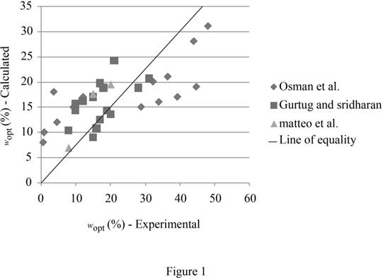
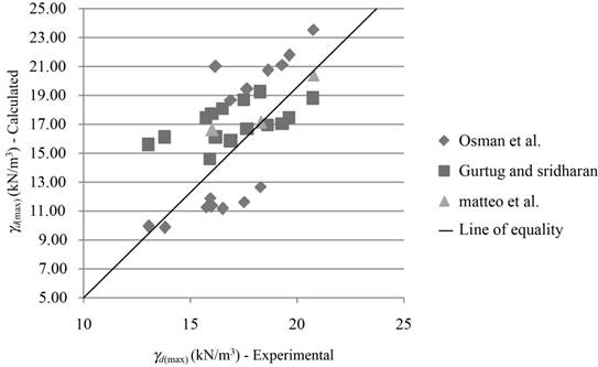
Plot the graph between the calculated wopt values versus experimental wopt values, and the calculated γd(max) values versus experimental γd(max) values. Draw the 45° line of equality on the each plot.
Explanation of Solution
Refer Table 1, 2, and 3.
Draw the graph between the calculated wopt values versus experimental wopt values as in Figure 1.
Draw the graph between calculated γd(max) values versus experimental γd(max) values as in Figure 2.
(e)
Comment on the predictive capabilities of various methods and comment about the inherent nature of empirical models.
Explanation of Solution
Prediction of optimum moisture content:
Refer Figure (1), several data points are closely packed around the 45° line for both the method of Osman et al. (2008) and Gurtug and Sridharan (2004) models signifying reasonable agreement between the calculated and experimental values. For the remaining soils, a poor agreement is observed. The one point from the Matteo method in the model plot showing the close agreement near the equality line and the other two points are slightly away from the equality line.
Prediction of maximum dry unit weight:
Most data points for all models show good covenant between the calculated and the experimental values.
The empirical models are often limited to the materials, test methods and environmental conditions under which the experiments were conducted and the developed models. For new materials and conditions, the predicted values may not be reliable.
Want to see more full solutions like this?
Chapter 6 Solutions
Principles Of Geotechnical Engineering, Si Edition


- From station 10+100 with center heights of 2 m in fill, the ground line makes a uniform slope of 4.8% to station 10+150 whose center heights is 1.2 m in cut. 1. Determine the slope of a new roadway to be constructed. 2. Determine the distance from station 10+150, will the excavation extend. 3. Determine the area of fill 10 m from 10+100 if the width of roadway is 8 m and the side slope is 1:2.arrow_forwardFunding Plan How much funds required to reach to the next level of the venture? • ? How much have been bootstrapped? If not, why? • ? How much can be bootstrapped? • ? How much external funding required? If not, why? • ? Funds utilization strategy (Details) • ? • ? • ? • ? • ? • ? • • ? ? ? ? ? Place your logo herearrow_forwardA semicircular 40 ft diameter− − tunnel is to be built under a150 ft deep− − , 800 ft long− − lake, as shown below. a) Determine the horizontal, vertical, and resulting hydrostatic forces acting on this tunnel. (Answer: 8 8 8 1.398 10 , 2.596 10 , 2.64 10H y netF lbf F lbf F lbf= × = × = × ) b) Calculate the hydrostatic force on the bottom of the lake if the tunnel was not there, and compare it with the total (resulting) hydrostatic force that you calculated in part (a). (Answer: 8 2.995 10VF lbf= × ) c) As the design engineer of this tunnel would you take the hydrostatic force on the bottom of the lake as a rough estimate of the resulting hydrostatic force acting on this tunnel. Discuss your decision.arrow_forward
- 3.2 Consi parabolic equation (Eq. 3.1) 3.3 Again consider Example 3.4. Does this curve provide sufficient stopping sight distance for a speed of 60 mi/h? -tangent grade with a -1% final mi/h. The station of the 1203 ft. What is the elev 3.4 An equal-tangent crest vertical curve is designed for 70 mi/h. The high point is at elevation 1011.4 ft. The initial grade is +2% and the final grade is -1%. What is the elevation of the PVT? +00? 3.10 An equal-tangent w 2012 (to 2011 AASHTO of 70 mi/h to connec -2.1%. The curve is design speed in th technology has adv design deceleration value used to dev percentage of ol design reaction vehicles have b height is assun roadway obje 3.5 An equal-tangent crest curve has been designed for 70 mi/h to connect a +2% initial grade and a -1% final grade for a new vehicle that has a 3 ft driver's eye height; the curve was designed to avoid an object that is 1 ft high. Standard practical stopping distance design was used but, unlike current design standards,…arrow_forwardFactor of Safety Activity The lap joint is connected by three 20-mm diameter rivets. Assuming that the applied allowable load, P=50kN is distributed equally among the three rivets and a factor of safety of 1.5, find: (a) the failure shear stress in a rivet, and (b) failure bearing stress between the plate and rivet 25 mm 25 mmarrow_forwardDraw the shear and moment diagrams of the beam CDE showing all calculations. Assume the support at A is a roller and B is a pin. There are fixed connected joints at D and E. Assume P equals 9.6 and w equals 0.36arrow_forward
- Find the length of the diagonal on the x-z plane (square root of square of sides). Find angle between the vector F and its projection on x-z (the diagonal defined above). Find Horizontal Projection of F on x-z plane, Fh, and vertical component, FY. Find projections of Fh, to define in-plane components Fx and Fz. Show that results match those of Problem 2(a) above. (2,0,4) F₂ 100 N (5, 1, 1)arrow_forwardFor the control system Draw Nyquist Plot with Solution G(S)= 63.625 (S+1)(S+3) S(S+2)(5+65+18) (5+5)arrow_forwardQ3: Find the support reactions at A: y mm A P=last 2 student's ID#+100 (N) 124N last 3 student's ID# (mm) 724mm 20 mm D B C X last 3 student's ID#+20 mm 744mm 40 mm 60 mmarrow_forward
- A hoist trolley is subjected to the three forces shown. Knowing that α = 40°, determine (a) the required magnitude of the force P if the resultant of the three forces is to be vertical, (b) the corresponding magnißide of the resultant. α 724lb last 3 student's ID# lb α last 2 student's ID#+100 lb 124lb Parrow_forwardFive wood boards are bolted together to form the built-up beam shown in the figure. The beam is subjected to a shear force of V = 13 kips. Each bolt has a shear strength of Vbolt = 6 kips. [h₁ =4.25 in., t₁ = 0.5 in., h₂ = 6 in., t₂ = 1 in.] hi + hi/2 h:/2 h: 2 h + h/2 Determine the moment of inertia of the section. Determine the maximum allowable spacing of the bolts. Determine the shear flow in the section connected by fasteners.arrow_forwardA vessel has a diameter of 1m and 2m high is moving downward with a positive acceleration of 3m/s2. The pressure at the bottom of the liquid is 9.534kPa, determine the mass of the liquid.arrow_forward
 Principles of Geotechnical Engineering (MindTap C...Civil EngineeringISBN:9781305970939Author:Braja M. Das, Khaled SobhanPublisher:Cengage Learning
 Fundamentals of Geotechnical Engineering (MindTap...Civil EngineeringISBN:9781305635180Author:Braja M. Das, Nagaratnam SivakuganPublisher:Cengage Learning
 Construction Materials, Methods and Techniques (M...Civil EngineeringISBN:9781305086272Author:William P. Spence, Eva KultermannPublisher:Cengage Learning
 Principles of Foundation Engineering (MindTap Cou...Civil EngineeringISBN:9781337705028Author:Braja M. Das, Nagaratnam SivakuganPublisher:Cengage Learning
 Principles of Foundation Engineering (MindTap Cou...Civil EngineeringISBN:9781305081550Author:Braja M. DasPublisher:Cengage Learning
 Traffic and Highway EngineeringCivil EngineeringISBN:9781305156241Author:Garber, Nicholas J.Publisher:Cengage Learning