Chapter 6, Problem 1DH

Break into small groups and discuss the following topics. Organize a brief outline in which you summarize the main points of your group discussion.

Iris setosa is a beautiful wildflower that is found in such diverse places as Alaska, the Gulf of St. Lawrence, much of North America, and even in English meadows and parks. R. A. Fisher, with his colleague Dr. Edgar Anderson, studied these flowers extensively. Dr. Anderson described how he collected information on irises:

I have studied such irises as I could get to see, in as great detail as possible, measuring iris standard after iris standard and iris fall after iris fall, sitting squat-legged with record book and ruler in mountain meadows, in cypress swamps, on lake beaches, and in English parks. [E. Anderson, “The Irises of the Gaspé Peninsula,” Bulletin, American Iris Society, Vol. 59 pp. 2–5, 1935.]

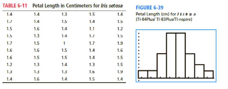
The data in Table 6-11 were collected by Dr. Anderson and were published by his friend and colleague R. A. Fisher in a paper titled “The Use of Multiple Measurements in Taxonomic Problems” (Annals of Eugenics, part II, pp. 179–188, 1936). To find these data, visit the Carnegie Mellon University Data and Story Library (DASL) web site. From the DASL site, look under Biology and Wild iris select Fisher's Irises Story.

Let x be a random variable representing petal length. Using a TI-84Plus/ TI-83Plus/TI-nspire calculator, it was found that the sample mean is $\bar{x}$ = 1.46 centimeters (cm) and the sample standard deviation is s = 0.17 cm. Figure 6-39 shows a histogram for the given data generated on a TI-84Plus/TI-83Plus/TI-nspire calculator.

1. (a) Examine the histogram for petal lengths. Would you say that the distribution is approximately mound-shaped and symmetric? Our sample has only 50 irises; if many thousands of irises had been used, do you think the distribution would look even more like a normal curve? Let x be the petal length of Iris setosa. Research has shown that x has an approximately normal distribution, with mean μ = 1.5 cm and standard deviation σ = 0.2 cm.
2. (b) Use the empirical rule with μ = 1.5 and σ = 0.2 to get an interval into which approximately 68% of the petal lengths will fall. Repeat this for 95% and 99.7%. Examine the raw data and compute the percentage of the raw data that actually fall into each of these intervals (the 68% interval, the 95% interval, and the 99.7% interval). Compare your computed percentages with those given by the empirical rule.
3. (c) Compute the probability that a petal length is between 1.3 and 1.6 cm. Compute the probability that a petal length is greater than 1.6 cm.
4. (d) Suppose that a random sample of 30 irises is obtained. Compute the probability that the average petal length for this sample is between 1.3 and 1.6 cm. Compute the probability that the average petal length is greater than 1.6 cm.
5. (e) Compare your answers to parts (c) and (d). Do you notice any differences? Why would these differences occur?

To determine

Explain whether the distribution is approximately mound-shaped and symmetrical.

Answer to Problem 1DH

Yes, the distribution is approximately mound-shaped and symmetrical.

Explanation of Solution

From the histogram for petal lengths, the distribution is approximately bell-shaped or mound-shaped and symmetrical because approximately the left half of the graph is the mirror image of the right half of the graph.

Our sample has only 50 irises; if many thousands of irises had been used, the distribution would look more similar to a normal curve because the sample is very large and the distribution of the sample will be approximately normally distributed.

To determine

Obtain the 68%, 95%, and 99% interval and compare the computed percentages with those given by the empirical rule.

Answer to Problem 1DH

The 68%, 95%, and 99% intervals are (1.3, 1.7), (1.1, 1.9), and (0.9, 2.1), respectively.

Explanation of Solution

Let x be the petal length of Iris Setosa and x has an approximately normal distribution, with mean $\mu =1.5$ cm and standard deviation $\sigma =0.2$ cm.

It is known that 68% of the observations will fall within one standard deviation of mean.

The 68% interval is as follows:

$\begin{array}{c}\left(\mu -\sigma , \mu +\sigma \right)=\left(1.5-0.2, 1.5+0.2\right)\\ =\left(1.3, 1.7\right)\end{array}$

The 95% of the observations will fall within two standard deviations of mean.

The 95% interval is as follows:

$\begin{array}{c}(\mu -2\sigma , \mu +2\sigma )=\left(1.5-2\left(0.2\right), 1.5+2\left(0.2\right)\right)\\ =\left(1.1, 1.9\right)\end{array}$

The 99.7% of the observations will fall within two standard deviations of mean.

The 99.7% interval is as follows:

$\begin{array}{c}\left(\mu -3\sigma , \mu +3\sigma \right)=\left(1.5-3\left(0.2\right), 1.5+3\left(0.2\right)\right)\\ =\left(0.9, 2.1\right)\end{array}$

The 33 observations fall within the intervals 1.3 and 1.7;thus, the percentage of data within the intervals 1.3 and 1.7 is $\frac{33}{50}=0.66$. This percentage is closer to 68%.

The 46 observations fall within the intervals 1.1 and 1.9;thus, the percentage of data within the intervals 1.3 and 1.7 is $\frac{46}{50}=0.92$. This percentage is closer to 95%.

All data values fall within the intervals 0.9 and 2.1;thus, the percentage of data within the intervals 1.3 and 1.7 is $\frac{50}{50}=1$. This percentage is closer to 99.7%.

To determine

Obtain the probability that a petal length is between 1.3 and 1.6 cm and the probability that a petal length is greater than 1.6 cm.

Answer to Problem 1DH

The probability that a petal length is between 1.3 and 1.6 cm is 0.5328.

The probability that a petal length is greater than 1.6 cm is 0.3085.

Explanation of Solution

Let x be the petal length of Iris Setosa and x has an approximately normal distribution, with mean $\mu =1.5$ cm and standard deviation $\sigma =0.2$ cm.

The interval $1.3\le x\le 1.6$ is converted to a corresponding interval on the standard z axis.

$\begin{array}{c}z=\frac{\left(x-\mu \right)}{\sigma }\\ =\frac{\left(x-1.5\right)}{0.2}\end{array}$

The z-score for $x=1.3$ is given below:

$\begin{array}{c}z=\frac{\left(1.3-1.5\right)}{0.2}\\ =-1\end{array}$

The z-score for $x=1.6$ is given below:

$\begin{array}{c}z=\frac{\left(1.6-1.5\right)}{0.2}\\ =0.5\end{array}$

The probabilitythat a petal length is between 1.3 and 1.6 cm is obtained as shown below:

$\begin{array}{c}P\left(1.3\le x\le 1.6\right)=P\left(-1\le z\le 0.5\right)\\ =P\left(z\le 0.5\right)-P\left(z\le -1\right)\end{array}$

In Appendix II, Table 5: Areas of a Standard Normal Distribution.

The values of $P(z\le 0.5)$ and $P(z\le -1)$ are obtained using the tables.

The probability corresponding to 0.5 is 0.6915 and the probability corresponding to -1 is 0.1587.

$\begin{array}{c}P\left(1.3\le x\le 1.6\right)=0.6915-0.1587\\ =0.5328\end{array}$

Hence, the probability that a petal length is between 1.3 and 1.6 cm is 0.5328.

The z-score for $x=1.6$ is given below:

$\begin{array}{c}z=\frac{\left(1.6-1.5\right)}{0.2}\\ =0.5\end{array}$

The probability that a petal length is greater than 1.6 cm is obtained as given below:

$\begin{array}{c}P\left(x>1.6\right)=P\left(z>0.5\right)\\ =1-P\left(z<0.5\right)\end{array}$

Using Table 5 from the Appendix, the probability corresponding to 0.5 is 0.6915.

$\begin{array}{c}P\left(x>1.6\right)=1-0.6915\\ =0.3085\end{array}$

Hence, the probability that a petal length is greater than 1.6 cm is 0.3085.

To determine

Obtain the probability that the average petal length is between 1.3 and 1.6 cm and the probability that the average petal length is greater than 1.6 cm.

Answer to Problem 1DH

The probability that the average petal length is between 1.3 and 1.6 cm is 0.9972.

The probability that the averagepetal length is greater than 1.6 cm is 0.0027.

Explanation of Solution

Let x be the petal length of Iris Setosa and x has an approximately normal distribution, with mean $\mu =1.5$ cm and standard deviation $\sigma =0.2$ cm.

With sample size as n = 30, the sampling distribution for $\overline{x}$ would be approximately normal with mean ${\mu }_{\overline{x}}$ and standard deviation ?${\sigma }_{\overline{x}}$.

$\begin{array}{c}{\mu }_{\overline{x}}=\mu \\ =1.5,\\ {\sigma }_{\overline{x}}=\frac{\sigma }{\sqrt{n}}\\ =\frac{0.2}{\sqrt{30}}\\ {\sigma }_{\overline{x}}=0.036\end{array}$

The interval $1.3\le \overline{x}\le 1.6$ is converted to a corresponding interval on the standard z axis.

$\begin{array}{c}z=\frac{\left(\overline{x}-{\mu }_{\overline{x}}\right)}{{\sigma }_{\overline{x}}}\\ =\frac{\left(\overline{x}-1.5\right)}{0.036}\end{array}$

The z-score for $\overline{x}=1.3$ is given below:

$\begin{array}{c}z=\frac{\left(1.3-1.5\right)}{0.036}\\ =-5.55\end{array}$

The z-score for $\overline{x}=1.6$ is given below:

$\begin{array}{c}z=\frac{\left(1.6-1.5\right)}{0.036}\\ =2.78\end{array}$

The probability that the average petal length is between 1.3 and 1.6 cm is obtained as shown below:

$\begin{array}{c}P\left(1.3\le \overline{x}\le 1.6\right)=P\left(-5.55\le z\le 2.78\right)\\ =P\left(z\le 2.78\right)-P\left(z\le -5.55\right)\end{array}$

In Appendix II, Table 5: Areas of a Standard Normal Distribution.

The values of $P(z\le 2.78)$ and $P(z\le -5.55)$ are obtained using the tables.

The probability corresponding to 2.78 is 0.9973 and the probability corresponding to -5.55does exist; Thus, it is considered as 0.0001.

$\begin{array}{c}P\left(1.3\le \overline{x}\le 1.6\right)=0.9973-0.0001\\ =0.9972\end{array}$

Hence, the probability that the average petal length is between 1.3 and 1.6 cm is 0.9972.

The z-score for $\overline{x}=1.6$ is given below:

$\begin{array}{c}z=\frac{\left(1.6-1.5\right)}{0.036}\\ =2.78\end{array}$

The probability that the average petal length is greater than 1.6 cm is obtained as given below:

$\begin{array}{c}P\left(\overline{x}>1.6\right)=P\left(z>2.78\right)\\ =1-P\left(z<2.78\right)\end{array}$

Using Table 5 from the Appendix, the probability corresponding to 2.78 is 0.9973.

$\begin{array}{c}P\left(\overline{x}>1.6\right)=1-0.9973\\ =0.0027\end{array}$

Hence, the probability that the average petal length is greater than 1.6 cm is 0.0027.

To determine

Compare the results of Part (c) and Part (d); also delineate the differences.

Answer to Problem 1DH

The standard deviation of the sample mean is much smaller than the population standard deviation.

Explanation of Solution

In Part (c), x has a distribution that is approximately normal with $\mu =1.5, \sigma =0.2$.

In Part (d), $\overline{x}$ is a sample mean corresponding to a random sample of size n = 30 taken from the x distribution whose mean ${\mu }_{\overline{x}}=1.5$ and standard deviation ?${\sigma }_{\overline{x}}=0.036$. Since the standard deviation for $\overline{x}$ distribution is much smaller than it is for the x distribution, the answers to Parts (c) and (d) are very different.

The central limit theorem tells us that the standard deviation of the sample mean is much smaller than the population standard deviation.