Concept explainers
Videos
Specialty Toys
Specialty Toys, Inc., sells a variety of new and innovative children’s toys. Management learned that the preholiday season is the best time to introduce a new toy, because many families use this time to look for new ideas for December holiday gifts. When Specialty discovers a new toy with good market potential, it chooses an October market entry date.
In order to get toys in its stores by October, Specialty places one-time orders with its manufacturers in June or July of each year. Demand for children’s toys can be highly volatile. If a new toy catches on, a sense of shortage in the marketplace often increases the demand to high levels and large profits can be realized. However, new toys can also flop, leaving Specialty stuck with high levels of inventory that must be sold at reduced prices. The most important question the company faces is deciding how many units of a new toy should be purchased to meet anticipated sales demand. If too few are purchased, sales will be lost; if too many are purchased, profits will be reduced because of low prices realized in clearance sales.
For the coming season, Specialty plans to introduce a new product called Weather Teddy. This variation of a talking teddy bear is made by a company in Taiwan. When a child presses Teddy’s hand, the bear begins to talk. A built-in barometer selects one of five responses that predict the weather conditions. The responses
As with other products, Specialty faces the decision of how many Weather Teddy units to order for the coming holiday season. Members of the management team suggested order quantities of 15,000, 18,000, 24,000, or 28,000 units. The wide range of order quantities suggested indicates considerable disagreement concerning the market potential. The product management team asks you for an analysis of the stock-out probabilities for various order quantities, an estimate of the profit potential, and to help make an order quantity recommendation. Specialty expects to sell Weather Teddy for $24 based on a cost of $16 per unit. If inventory remains after the holiday season, Specialty will sell all surplus inventory for $5 per unit. After reviewing the sales history of similar products, Specialty’s senior sales forecaster predicted an expected demand of 20,000 units with a .95
Prepare a managerial report that addresses the following issues and recommends an order quantity for the Weather Teddy product.
- 1. Use the sales forecaster’s prediction to describe a
normal probability distribution that can be used to approximate the demand distribution. Sketch the distribution and show its mean and standard deviation. - 2. Compute the probability of a stock-out for the order quantities suggested by members of the management team.
- 3. Compute the projected profit for the order quantities suggested by the management team under three scenarios: worst case in which sales = 10,000 units, most likely case in which sales = 20,000 units, and best case in which sales = 30,000 units.
- 4. One of Specialty’s managers felt that the profit potential was so great that the order quantity should have a 70% chance of meeting demand and only a 30% chance of any stock-outs. What quantity would be ordered under this policy, and what is the projected profit under the three sales scenarios?
- 5. Provide your own recommendation for an order quantity and note the associated profit projections. Provide a rationale for your recommendation.
1.
Describe a normal probability distribution that can be used to approximate the demand distribution using the sales forecaster’s prediction.
Sketch the distribution and show its mean and standard deviation.
Answer to Problem 1CP
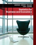
The normal distribution with a mean of 20,000 and a standard deviation of 5,102 can be used to approximate the demand distribution using the sales forecaster’s prediction.
The normal probability distribution that can be used to approximate the demand distribution is shown below:
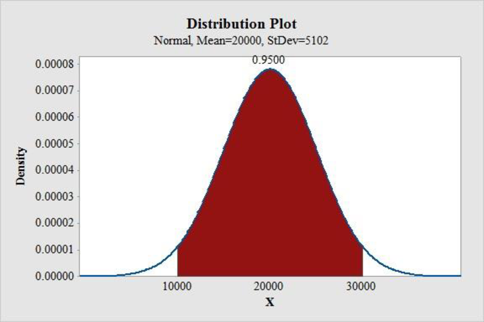
Figure (1)
Explanation of Solution
Calculation:
The order quantities suggested are 15,000, 18,000, 24,000 or 28,000 units. The Weather Teddy is expected to be sold at $24 based on a cost of $16 per unit. All surplus inventories are sold at a cost of $5 per unit. The sales forecaster’s predicted that there will be an expected demand of 20,000 units with a 0.95 probability that demand would be between 10,000 units and 30,000 units.
Define the random variable x as the demand.
From the information provided by the forecaster, demand would be between 10,000 units and 30,000 units with a 0.95 probability.
Software Procedure:
Step-by-step procedure to obtain the z-values using the MINITAB software:
- Choose Graph > Probability Distribution Plot.
- Choose View Probability > OK.
- From Distribution, choose ‘Normal’ distribution.
- Enter the Mean as 0 and Standard deviation as 1.
- Click the Shaded Area tab.
- Choose Probability and Both Tails for the region of the curve to shade.
- Enter the Probability value as 0.05.
- Click OK.
Output using the MINITAB software is given below:
From the MINITAB output the z-values are –1.96 and 1.96.
The formula for z-score is,
At
Thus, the normal distribution with a mean of 20,000 and a standard deviation of 5,102 can be used to approximate the demand distribution using the sales forecaster’s prediction.
Software Procedure:
Step-by-step procedure to draw the normal curve using the MINITAB software:
- Choose Graph > Probability Distribution Plot.
- Choose View Probability > OK.
- From Distribution, choose ‘Normal’ distribution.
- Enter the Mean as 20,000 and Standard deviation as 5,102.
- Click the Shaded Area tab.
- Choose X value and Middle area for the region of the curve to shade.
- Enter the as 0.05.
- Click OK.
The normal curve for demand is shown in figure (1).
2.
Find the probability of a stock-out for the order quantities suggested by members of the management team.
Answer to Problem 1CP
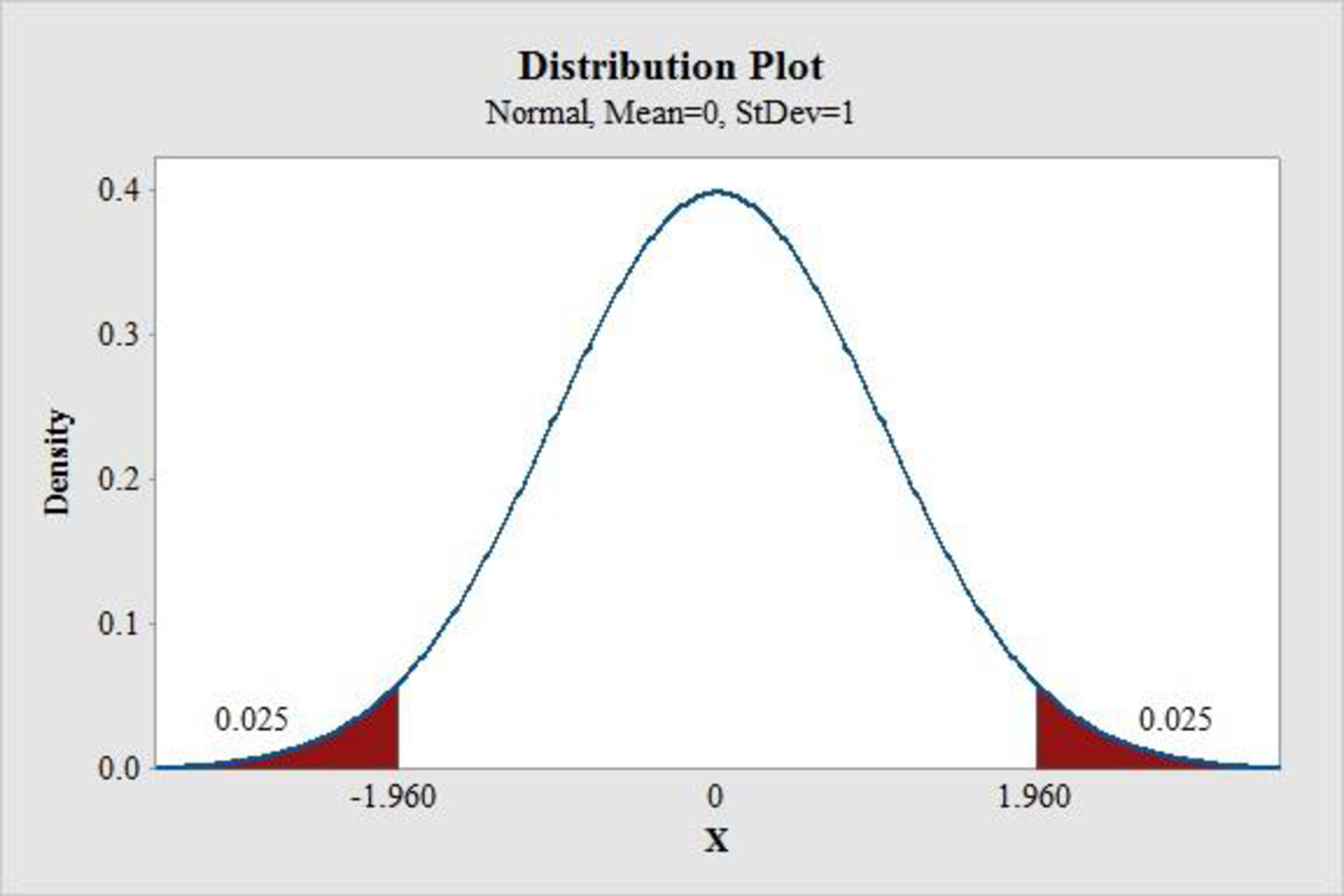
The probability of a stock-out for the order quantity of 15,000 units is 0.8365.
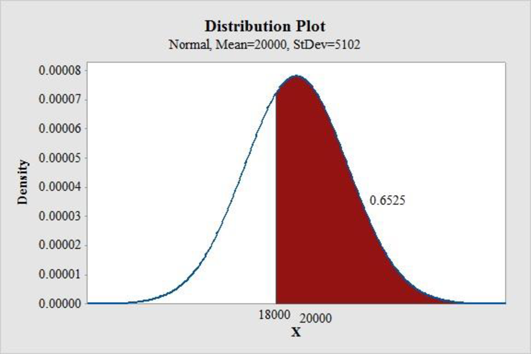
The probability of a stock-out for the order quantity of 18,000 units is 0.6525.
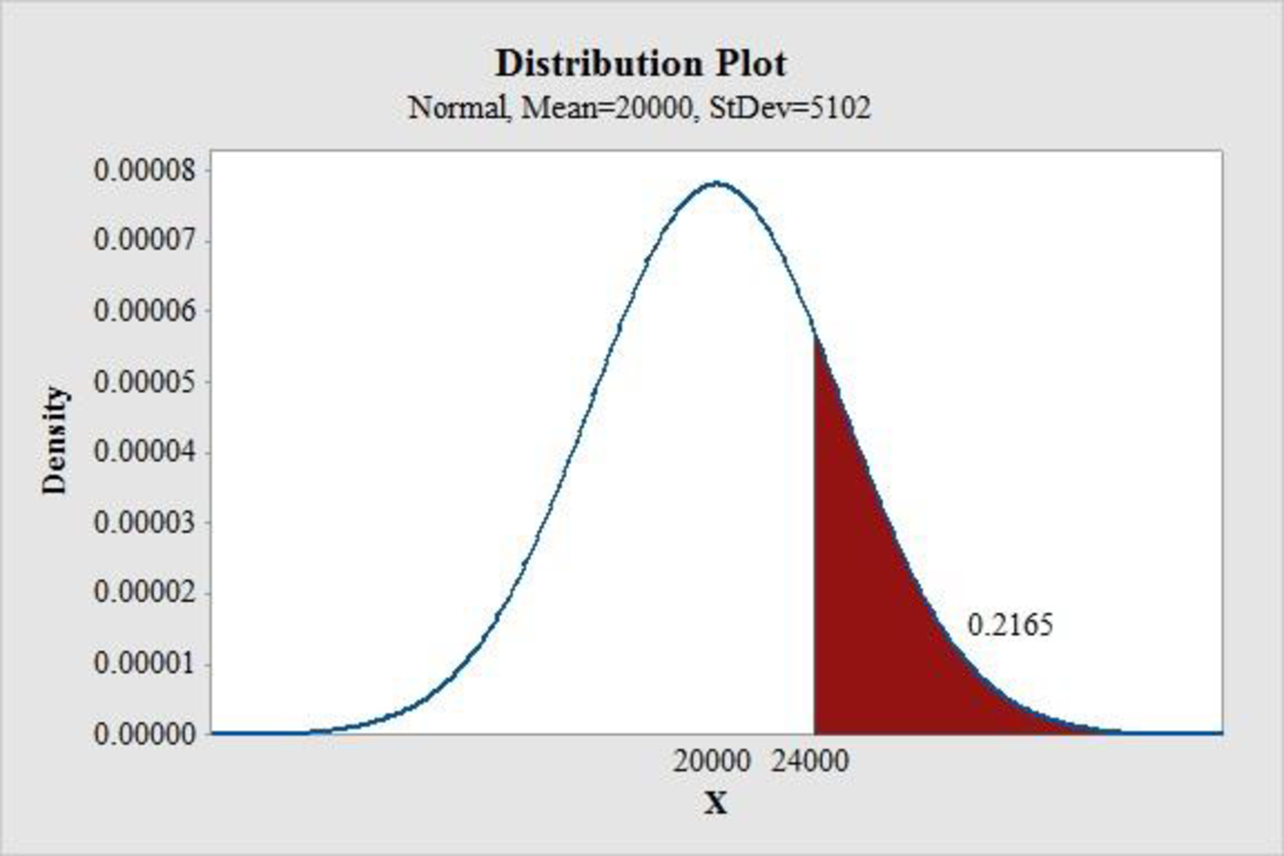
The probability of a stock-out for the order quantity of 24,000 units is 0.2165.
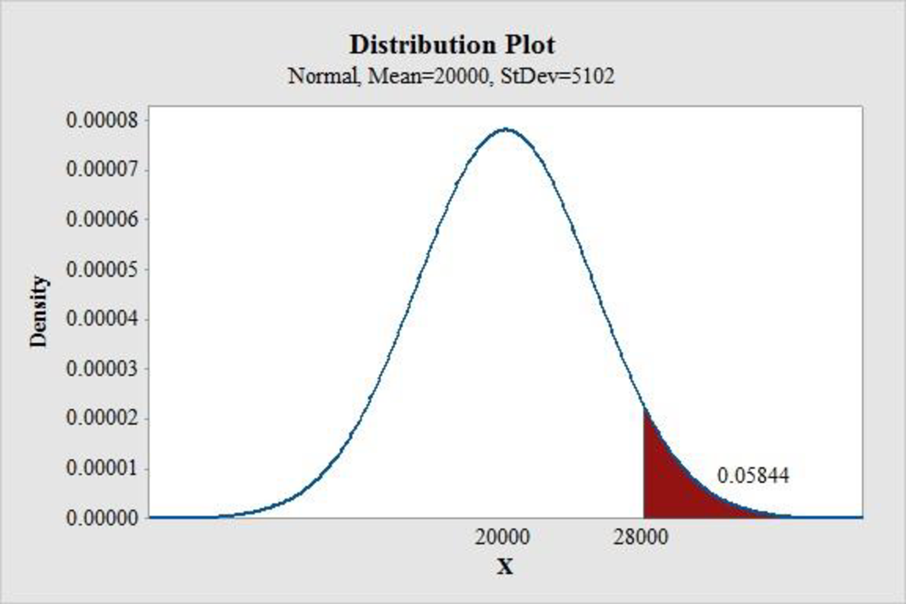
The probability of a stock-out for the order quantity of 28,000 units is 0.05844.
Explanation of Solution
Calculation:
The probability of a stock-out for the order quantity of 15,000 units is
Software Procedure:
Step-by-step procedure to obtain the probability value using the MINITAB software:
- Choose Graph > Probability Distribution Plot
- Choose View Probability > OK.
- From Distribution, choose ‘Normal’ distribution.
- Enter the Mean as 20,000 and Standard deviation as 5,102.
- Click the Shaded Area tab.
- Choose X Value and Right Tail for the region of the curve to shade.
- Enter the X value as 15,000.
- Click OK.
Output using the MINITAB software is given below:
From the MINITAB output,
Thus, the probability of a stock-out for the order quantity of 15,000 units is 0.8365.
The probability of a stock-out for the order quantity of 18,000 units is
Software Procedure:
Step-by-step procedure to obtain the probability value using the MINITAB software:
- Choose Graph > Probability Distribution Plot
- Choose View Probability > OK.
- From Distribution, choose ‘Normal’ distribution.
- Enter the Mean as 20,000 and Standard deviation as 5,102.
- Click the Shaded Area tab.
- Choose X Value and Right Tail for the region of the curve to shade.
- Enter the X value as 18,000.
- Click OK.
Output using the MINITAB software is given below:
From the MINITAB output,
Thus, the probability of a stock-out for the order quantity of 18,000 units is 0.6525.
The probability of a stock-out for the order quantity of 24,000 units is
Software Procedure:
Step-by-step procedure to obtain the probability value using the MINITAB software:
- Choose Graph > Probability Distribution Plot
- Choose View Probability > OK.
- From Distribution, choose ‘Normal’ distribution.
- Enter the Mean as 20,000 and Standard deviation as 5,102.
- Click the Shaded Area tab.
- Choose X Value and Right Tail for the region of the curve to shade.
- Enter the X value as 24,000.
- Click OK.
Output using the MINITAB software is given below:
From the MINITAB output,
Thus, the probability of a stock-out for the order quantity of 24,000 units is 0.2165.
The probability of a stock-out for the order quantity of 28,000 units is
Software Procedure:
Step-by-step procedure to obtain the probability value using the MINITAB software:
- Choose Graph > Probability Distribution Plot
- Choose View Probability > OK.
- From Distribution, choose ‘Normal’ distribution.
- Enter the Mean as 20,000 and Standard deviation as 5,102.
- Click the Shaded Area tab.
- Choose X Value and Right Tail for the region of the curve to shade.
- Enter the X value as 28,000.
- Click OK.
Output using the MINITAB software is given below:
From the MINITAB output,
Thus, the probability of a stock-out for the order quantity of 28,000 units is 0.05844.
3.
Find the projected profit for the order quantities suggested by the management team under the three scenarios.
Answer to Problem 1CP
The projected profit for the order quantities are given below:
For an order quantity of 15,000 units:
| Unit sales | Total cost ($) | At $24 | At $5 | Profit($) |
| 10,000 | 240,000 | 240,000 | 25,000 | 25,000 |
| 20,000 | 240,000 | 360,000 | 0 | 120,000 |
| 30,000 | 240,000 | 360,000 | 0 | 120,000 |
For an order quantity of 18,000 units:
| Unit sales | Total cost ($) | At $24 | At $5 | Profit($) |
| 10,000 | 288,000 | 240,000 | 40,000 | –8,000 |
| 20,000 | 288,000 | 432,000 | 0 | 144,000 |
| 30,000 | 288,000 | 432,000 | 0 | 144,000 |
For an order quantity of 24,000 units:
| Unit sales | Total cost ($) | At $24 | At $5 | Profit($) |
| 10,000 | 384,000 | 240,000 | 70,000 | –74,000 |
| 20,000 | 384,000 | 480,000 | 20,000 | 116,000 |
| 30,000 | 384,000 | 576,000 | 0 | 192,000 |
For an order quantity of 28,000 units:
| Unit sales | Total cost ($) | At $24 | At $5 | Profit($) |
| 10,000 | 448,000 | 240,000 | 90,000 | –118,000 |
| 20,000 | 448,000 | 480,000 | 40,000 | 72,000 |
| 30,000 | 448,000 | 672,000 | 0 | 224,000 |
Explanation of Solution
Calculation:
The three scenarios under consideration are, worst case in which there is a sale of 10,000 units, most likely case in which there is a sale of 20,000 units and the best case in which there is a sale of 30,000 units.
The profit projections for the order quantities under three scenarios are computed using the following table:
For an order quantity of 15,000 units:
Total cost is obtained by multiplying the cost of a unit ($16) with the order quantity.
The income at $24 is obtained by multiplying $24 with the number of units sold.
For the unit sales more than 15, 000, the income at $24 is obtained by multiplying $24 with the order quantity 15,000 units.
The income at $5 is obtained by multiplying $5 with the number of surplus units (number of units sold–order quantity).
The income at $5 will be zero for the order quantities more than 15,000 units.
The profit is obtained as shown below:
Profit obtained for a sale of 10,000 units is,
| Unit sales | Total cost ($) | At $24 | At $5 | Profit($) |
| 10,000 | 240,000 | 240,000 | 25,000 | 25,000 |
| 20,000 | 240,000 | 360,000 | 0 | 120,000 |
| 30,000 | 240,000 | 360,000 | 0 | 120,000 |
Similarly, the profit projections are obtained and are given in the following tables:
For an order quantity of 18,000 units:
| Unit sales | Total cost ($) | At $24 | At $5 | Profit($) |
| 10,000 | 288,000 | 240,000 | 40,000 | –8,000 |
| 20,000 | 288,000 | 432,000 | 0 | 144,000 |
| 30,000 | 288,000 | 432,000 | 0 | 144,000 |
For an order quantity of 24,000 units:
| Unit sales | Total cost ($) | At $24 | At $5 | Profit($) |
| 10,000 | 384,000 | 240,000 | 70,000 | –74,000 |
| 20,000 | 384,000 | 480,000 | 20,000 | 116,000 |
| 30,000 | 384,000 | 576,000 | 0 | 192,000 |
For an order quantity of 28,000 units:
| Unit sales | Total cost ($) | At $24 | At $5 | Profit($) |
| 10,000 | 448,000 | 240,000 | 90,000 | –118,000 |
| 20,000 | 448,000 | 480,000 | 40,000 | 72,000 |
| 30,000 | 448,000 | 672,000 | 0 | 224,000 |
4.
Find quantity that would be ordered under the policy and the profit at three sales scenarios.
Answer to Problem 1CP
The quantity that would be ordered under the policy is 22,675.
The profit at three sales scenarios are given in the following table:
| Unit sales | Total cost ($) | At $24 | At $5 | Profit($) |
| 10,000 | 362,800 | 240,000 | 63,375 | –59,425 |
| 20,000 | 362,800 | 480,000 | 13,375 | 130,575 |
| 30,000 | 362,800 | 544,200 | 0 | 181,400 |
Explanation of Solution
Calculation:
The order quantity should have a 70% chance of meeting demand and only a 30% chance of any stock outs. That is the order quantity that cuts off an area of 0.70 in the lower tail of the normal curve for demand.
Software Procedure:
Step-by-step procedure to obtain the x value using the MINITAB software:
- Choose Graph > Probability Distribution Plot.
- Choose View Probability > OK.
- From Distribution, choose ‘Normal’ distribution.
- Enter the Mean as 20,000 and Standard deviation as 5,102.
- Click the Shaded Area tab.
- Choose Probability Value and left tail for the region of the curve to shade.
- Enter the Probability value as 0.70.
- Click OK.
Output using the MINITAB software is given below:
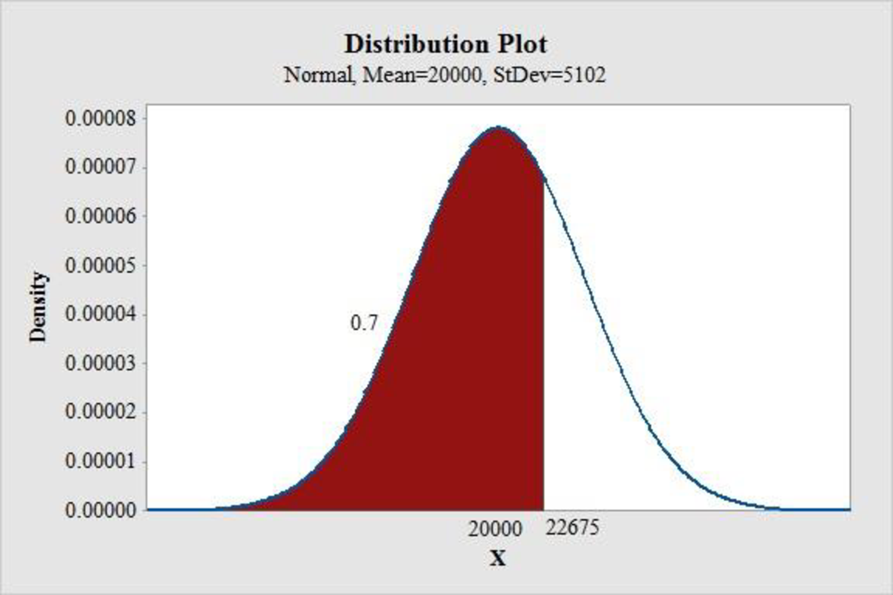
Thus, the quantity that would be ordered under the policy is 22,675.
The profit projections are obtained with the similar calculations made in part(c) for an order quantity of 22,675 units and is given in the following table:
| Unit sales | Total cost ($) | At $24 | At $5 | Profit($) |
| 10,000 | 362,800 | 240,000 | 63,375 | –59,425 |
| 20,000 | 362,800 | 480,000 | 13,375 | 130,575 |
| 30,000 | 362,800 | 544,200 | 0 | 181,400 |
5.
Provide the recommendation for an order quantity and note the associated profit projections and provide the rationale for the recommendation.
Explanation of Solution
A variety of recommendations are possible. From the three scenarios used in part (c) and (d) it is clear that an order quantity in the range 18,000 to 20,000 will be good to generate profit. Because the order quantities of more than 20,000 units generates a risk of loss and reduces the chance of generating good profits.
Want to see more full solutions like this?
Chapter 6 Solutions
EBK STATISTICS FOR BUSINESS & ECONOMICS


- Question 1 The data shown in Table 1 are and R values for 24 samples of size n = 5 taken from a process producing bearings. The measurements are made on the inside diameter of the bearing, with only the last three decimals recorded (i.e., 34.5 should be 0.50345). Table 1: Bearing Diameter Data Sample Number I R Sample Number I R 1 34.5 3 13 35.4 8 2 34.2 4 14 34.0 6 3 31.6 4 15 37.1 5 4 31.5 4 16 34.9 7 5 35.0 5 17 33.5 4 6 34.1 6 18 31.7 3 7 32.6 4 19 34.0 8 8 33.8 3 20 35.1 9 34.8 7 21 33.7 2 10 33.6 8 22 32.8 1 11 31.9 3 23 33.5 3 12 38.6 9 24 34.2 2 (a) Set up and R charts on this process. Does the process seem to be in statistical control? If necessary, revise the trial control limits. [15 pts] (b) If specifications on this diameter are 0.5030±0.0010, find the percentage of nonconforming bearings pro- duced by this process. Assume that diameter is normally distributed. [10 pts] 1arrow_forward4. (5 pts) Conduct a chi-square contingency test (test of independence) to assess whether there is an association between the behavior of the elderly person (did not stop to talk, did stop to talk) and their likelihood of falling. Below, please state your null and alternative hypotheses, calculate your expected values and write them in the table, compute the test statistic, test the null by comparing your test statistic to the critical value in Table A (p. 713-714) of your textbook and/or estimating the P-value, and provide your conclusions in written form. Make sure to show your work. Did not stop walking to talk Stopped walking to talk Suffered a fall 12 11 Totals 23 Did not suffer a fall | 2 Totals 35 37 14 46 60 Tarrow_forwardQuestion 2 Parts manufactured by an injection molding process are subjected to a compressive strength test. Twenty samples of five parts each are collected, and the compressive strengths (in psi) are shown in Table 2. Table 2: Strength Data for Question 2 Sample Number x1 x2 23 x4 x5 R 1 83.0 2 88.6 78.3 78.8 3 85.7 75.8 84.3 81.2 78.7 75.7 77.0 71.0 84.2 81.0 79.1 7.3 80.2 17.6 75.2 80.4 10.4 4 80.8 74.4 82.5 74.1 75.7 77.5 8.4 5 83.4 78.4 82.6 78.2 78.9 80.3 5.2 File Preview 6 75.3 79.9 87.3 89.7 81.8 82.8 14.5 7 74.5 78.0 80.8 73.4 79.7 77.3 7.4 8 79.2 84.4 81.5 86.0 74.5 81.1 11.4 9 80.5 86.2 76.2 64.1 80.2 81.4 9.9 10 75.7 75.2 71.1 82.1 74.3 75.7 10.9 11 80.0 81.5 78.4 73.8 78.1 78.4 7.7 12 80.6 81.8 79.3 73.8 81.7 79.4 8.0 13 82.7 81.3 79.1 82.0 79.5 80.9 3.6 14 79.2 74.9 78.6 77.7 75.3 77.1 4.3 15 85.5 82.1 82.8 73.4 71.7 79.1 13.8 16 78.8 79.6 80.2 79.1 80.8 79.7 2.0 17 82.1 78.2 18 84.5 76.9 75.5 83.5 81.2 19 79.0 77.8 20 84.5 73.1 78.2 82.1 79.2 81.1 7.6 81.2 84.4 81.6 80.8…arrow_forward
- Name: Lab Time: Quiz 7 & 8 (Take Home) - due Wednesday, Feb. 26 Contingency Analysis (Ch. 9) In lab 5, part 3, you will create a mosaic plot and conducted a chi-square contingency test to evaluate whether elderly patients who did not stop walking to talk (vs. those who did stop) were more likely to suffer a fall in the next six months. I have tabulated the data below. Answer the questions below. Please show your calculations on this or a separate sheet. Did not stop walking to talk Stopped walking to talk Totals Suffered a fall Did not suffer a fall Totals 12 11 23 2 35 37 14 14 46 60 Quiz 7: 1. (2 pts) Compute the odds of falling for each group. Compute the odds ratio for those who did not stop walking vs. those who did stop walking. Interpret your result verbally.arrow_forwardSolve please and thank you!arrow_forward7. In a 2011 article, M. Radelet and G. Pierce reported a logistic prediction equation for the death penalty verdicts in North Carolina. Let Y denote whether a subject convicted of murder received the death penalty (1=yes), for the defendant's race h (h1, black; h = 2, white), victim's race i (i = 1, black; i = 2, white), and number of additional factors j (j = 0, 1, 2). For the model logit[P(Y = 1)] = a + ß₁₂ + By + B²², they reported = -5.26, D â BD = 0, BD = 0.17, BY = 0, BY = 0.91, B = 0, B = 2.02, B = 3.98. (a) Estimate the probability of receiving the death penalty for the group most likely to receive it. [4 pts] (b) If, instead, parameters used constraints 3D = BY = 35 = 0, report the esti- mates. [3 pts] h (c) If, instead, parameters used constraints Σ₁ = Σ₁ BY = Σ; B = 0, report the estimates. [3 pts] Hint the probabilities, odds and odds ratios do not change with constraints.arrow_forward
- Solve please and thank you!arrow_forwardSolve please and thank you!arrow_forwardQuestion 1:We want to evaluate the impact on the monetary economy for a company of two types of strategy (competitive strategy, cooperative strategy) adopted by buyers.Competitive strategy: strategy characterized by firm behavior aimed at obtaining concessions from the buyer.Cooperative strategy: a strategy based on a problem-solving negotiating attitude, with a high level of trust and cooperation.A random sample of 17 buyers took part in a negotiation experiment in which 9 buyers adopted the competitive strategy, and the other 8 the cooperative strategy. The savings obtained for each group of buyers are presented in the pdf that i sent: For this problem, we assume that the samples are random and come from two normal populations of unknown but equal variances.According to the theory, the average saving of buyers adopting a competitive strategy will be lower than that of buyers adopting a cooperative strategy.a) Specify the population identifications and the hypotheses H0 and H1…arrow_forward
- You assume that the annual incomes for certain workers are normal with a mean of $28,500 and a standard deviation of $2,400. What’s the chance that a randomly selected employee makes more than $30,000?What’s the chance that 36 randomly selected employees make more than $30,000, on average?arrow_forwardWhat’s the chance that a fair coin comes up heads more than 60 times when you toss it 100 times?arrow_forwardSuppose that you have a normal population of quiz scores with mean 40 and standard deviation 10. Select a random sample of 40. What’s the chance that the mean of the quiz scores won’t exceed 45?Select one individual from the population. What’s the chance that his/her quiz score won’t exceed 45?arrow_forward
 MATLAB: An Introduction with ApplicationsStatisticsISBN:9781119256830Author:Amos GilatPublisher:John Wiley & Sons Inc
 Probability and Statistics for Engineering and th...StatisticsISBN:9781305251809Author:Jay L. DevorePublisher:Cengage Learning
 Statistics for The Behavioral Sciences (MindTap C...StatisticsISBN:9781305504912Author:Frederick J Gravetter, Larry B. WallnauPublisher:Cengage Learning
 Elementary Statistics: Picturing the World (7th E...StatisticsISBN:9780134683416Author:Ron Larson, Betsy FarberPublisher:PEARSON
 The Basic Practice of StatisticsStatisticsISBN:9781319042578Author:David S. Moore, William I. Notz, Michael A. FlignerPublisher:W. H. Freeman
 Introduction to the Practice of StatisticsStatisticsISBN:9781319013387Author:David S. Moore, George P. McCabe, Bruce A. CraigPublisher:W. H. Freeman