Videos
(a)
To find: The
(a)
Answer to Problem 78E
Solution: The mean and standard deviation of the binomial random variable X is 996 and 13.012 respectively.
Explanation of Solution
Calculation: In binomial distribution, the mean can be calculated by this formula,
In binomial distribution, standard deviation can be calculated by this formula,
Where, n is the number of trials and p is the
The standard deviation is calculated as:
Hence, the average value and standard deviation are 996 and 13.012 respectively.
(b)
To find: The probability.
(b)
Answer to Problem 78E
Solution: The probability is
Explanation of Solution
Calculation: The binomial random variable approximately follows the
Therefore, the random variable X can be approximated to normal distribution because the given condition is fulfilled.
The parameters of the normal distribution are calculated as follows:
And:
The probability that the value taken by X is greater than or equal to 800 is the area right to the point 800 under the normal curve. To obtain the area lying to the left of a point under the normal curve, first, convert the value of the variable into Z-score and then obtain the area lying to the right by subtracting the area left to the Z-score from 1. The Z-score for the value
The area left to the particular Z-score can be obtained using Excel by using the command
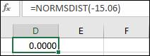
The area left to the Z-score,
So, the required probability can be calculated as:
Hence, the probability is 1.
(c)
To find: The probability.
(c)
Answer to Problem 78E
Solution:
Explanation of Solution
Calculation: For the probability that more than 1000 candidates will accept the admission, Excel has to be used. The following procedure is followed in Excel:
Step 1: Open the Excel spreadsheet.
Step 2: Type the command
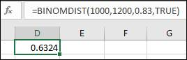
Therefore, the required probability is calculated as:
Hence, the probability is 0.3676.
(d)
To find: The probability.
(d)
Answer to Problem 78E
Solution:
Explanation of Solution
Calculation: The probability that more than 1000 candidates will accept the admission, Excel has to be used. The following procedure is followed in Excel:
Step 1: Open the Excel spreadsheet.
Step 2: Type the command
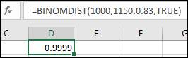
Therefore, the required probability is calculated as:
Hence, the probability is 0.0001.
Want to see more full solutions like this?
Chapter 5 Solutions
Introduction to the Practice of Statistics


- Business Discussarrow_forwardThe following data represent total ventilation measured in liters of air per minute per square meter of body area for two independent (and randomly chosen) samples. Analyze these data using the appropriate non-parametric hypothesis testarrow_forwardeach column represents before & after measurements on the same individual. Analyze with the appropriate non-parametric hypothesis test for a paired design.arrow_forward
- Should you be confident in applying your regression equation to estimate the heart rate of a python at 35°C? Why or why not?arrow_forwardGiven your fitted regression line, what would be the residual for snake #5 (10 C)?arrow_forwardCalculate the 95% confidence interval around your estimate of r using Fisher’s z-transformation. In your final answer, make sure to back-transform to the original units.arrow_forward
 MATLAB: An Introduction with ApplicationsStatisticsISBN:9781119256830Author:Amos GilatPublisher:John Wiley & Sons Inc
 Probability and Statistics for Engineering and th...StatisticsISBN:9781305251809Author:Jay L. DevorePublisher:Cengage Learning
 Statistics for The Behavioral Sciences (MindTap C...StatisticsISBN:9781305504912Author:Frederick J Gravetter, Larry B. WallnauPublisher:Cengage Learning
 Elementary Statistics: Picturing the World (7th E...StatisticsISBN:9780134683416Author:Ron Larson, Betsy FarberPublisher:PEARSON
 The Basic Practice of StatisticsStatisticsISBN:9781319042578Author:David S. Moore, William I. Notz, Michael A. FlignerPublisher:W. H. Freeman
 Introduction to the Practice of StatisticsStatisticsISBN:9781319013387Author:David S. Moore, George P. McCabe, Bruce A. CraigPublisher:W. H. Freeman