Concept explainers
Videos
(a)
To find: The
To find: The least-squares regression line for all four data sets.
To find: The predicted value for
(a)
Answer to Problem 5.42E
The correlation for the data set A is 0.816.
The correlation for the data set B is 0.816.
The correlation for the data set C is 0.816.
The correlation for the data set D is 0.8176.
The least-squares regression line for the data set A is
The least-squares regression line for the data set B is
The least-squares regression line for the data set C is
The least-squares regression line for the data set D is
The predicted value for
The predicted value for
The predicted value for
The predicted value for
Explanation of Solution
Given info:
The four data sets are used to exploring the
Calculation:
Correlation for Data set A:
Software procedure:
Step-by-step procedure to find the correlation between the x and y for data set A by using the MINITAB software:
- Select Stat >Basic Statistics > Correlation.
- In Variables, select x and y.
- Click OK.
Output using the MINITAB software is given below:
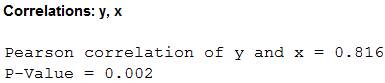
From the MINITAB output, the correlation between the x and y for data set A is 0.816.
Correlation for Data set B:
Software procedure:
Step-by-step procedure to find the correlation between the x and y for data set B by using the MINITAB software:
- Select Stat >Basic Statistics > Correlation.
- In Variables, select x and y.
- Click OK.
Output using the MINITAB software is given below:
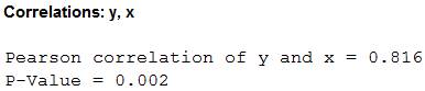
From the MINITAB output, the correlation between the x and y for data set B is 0.816.
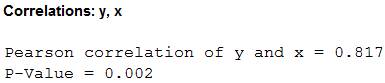
Correlation for Data set C:
Software procedure:
Step-by-step procedure to find the correlation between the x and y for data set C by using the MINITAB software:
- Select Stat >Basic Statistics > Correlation.
- In Variables, select x and y.
- Click OK.
Output using the MINITAB software is given below:
From the MINITAB output, the correlation between the x and y for data set C is 0.816.
Correlation for Data set D:
Software procedure:
Step-by-step procedure to find the correlation between the x and y for data set D by using the MINITAB software:
- Select Stat >Basic Statistics > Correlation.
- In Variables, select x and y.
- Click OK.
Output using the MINITAB software is given below:
From the MINITAB output, the correlation between the x and y for data set D is 0.817.
Equation of the least-squares line for Data set A:
Software procedure:
Step-by-step procedure to find the equation of the least-squares line by using the MINITAB software:
- Choose Stat > Regression > Regression.
- In Responses, enter the column of y.
- In Predictors, enter the column of x.
- Click OK.
Output using the MINITAB software is given below:
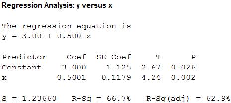
From the MINITAB output, the least-squares line for predicting y from x for data set A is
Equation of the least-squares line for Data set B:
Software procedure:
Step-by-step procedure to find the equation of the least-squares line by using the MINITAB software:
- Choose Stat > Regression > Regression.
- In Responses, enter the column of y.
- In Predictors, enter the column of x.
- Click OK.
Output using the MINITAB software is given below:
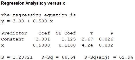
From the MINITAB output, the least-squares line for predicting y from x for data set B is
Equation of the least-squares line for Data set C:
Software procedure:
Step-by-step procedure to find the equation of the least-squares line by using the MINITAB software:
- Choose Stat > Regression > Regression.
- In Responses, enter the column of y.
- In Predictors, enter the column of x.
- Click OK.
Output using the MINITAB software is given below:
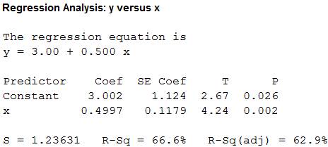
From the MINITAB output, the least-squares line for predicting y from x for data set C is
Equation of the least-squares line for Data set D:
Software procedure:
Step-by-step procedure to find the equation of the least-squares line by using the MINITAB software:
- Choose Stat > Regression > Regression.
- In Responses, enter the column of y.
- In Predictors, enter the column of x.
- Click OK.
Output using the MINITAB software is given below:
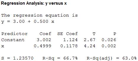
From the MINITAB output, the least-squares line for predicting y from x for data set D is
Predicted value for
Software procedure:
Step-by-step procedure to find the predicted value for
- Choose Stat > Regression > Regression.
- In Responses, enter the column of y.
- In Predictors, enter the column of x.
- In option, enter 10 under prediction.
- Click OK.
Output using the MINITAB software is given below:
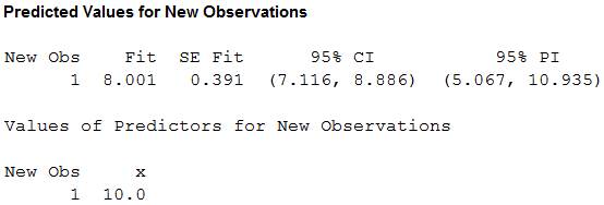
From the MINITAB output, the predicted value for
Predicted value for
Software procedure:
Step-by-step procedure to find the predicted value for
- Choose Stat > Regression > Regression.
- In Responses, enter the column of y.
- In Predictors, enter the column of x.
- In option, enter 10 under prediction.
- Click OK.
Output using the MINITAB software is given below:
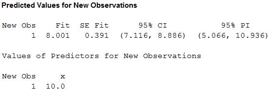
From the MINITAB output, the predicted value for
Predicted value for
Software procedure:
Step-by-step procedure to find the predicted value for
- Choose Stat > Regression > Regression.
- In Responses, enter the column of y.
- In Predictors, enter the column of x.
- In option, enter 10 under prediction.
- Click OK.
Output using the MINITAB software is given below:
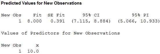
From the MINITAB output, the predicted value for
Predicted value for
Software procedure:
Step-by-step procedure to find the predicted value for
- Choose Stat > Regression > Regression.
- In Responses, enter the column of y.
- In Predictors, enter the column of x.
- In option, enter 10 under prediction.
- Click OK.
Output using the MINITAB software is given below:
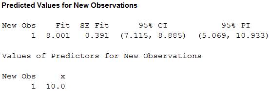
From the MINITAB output, the predicted value for
From the results, it can be observed that the correlation for all four data sets, the least-squares regression line and the predicted value for
(b)
To construct: The
(b)
Answer to Problem 5.42E
Scatterplot for Data set A:
Output using the MINITAB software is given below:
Scatterplot for Data set B:
Output using the MINITAB software is given below:
Scatterplot for Data set C:
Output using the MINITAB software is given below:
Scatterplot for Data set D:
Output using the MINITAB software is given below:
Explanation of Solution
Calculation:
Scatterplot:
Software procedure:
Step-by-step procedure to construct scatterplot for x and y for all four data sets by using the MINITAB software:
- Choose Graph > Scatter plot.
- Choose With Regression, and then click OK.
- Under Y variables, enter a column of y.
- Under X variables, enter a column of x.
- Click OK.
Observation:
The scatterplot shows that the predicted values are passed through the regression line of the model. Moreover, there is outlier that appears in the x and y directions for the data set A, B, and C. Also, the scatterplot for the data set D shows that the most of the points are plotted around 8.
(c)
To identify: Which of the four cases would you be willing to use the regression line to describe the dependence of y on x.
(c)
Answer to Problem 5.42E
The data set A would use the regression line to describe the dependence of y on x.
Explanation of Solution
From the scatterplots for all data sets, it can be observed that the points for data set A are scattered around the straight line when compared to the other data sets. Hence, the data set A would use the regression line to describe the dependence of y on x.
Want to see more full solutions like this?
Chapter 5 Solutions
BASIC PRACTICE OF STATS-LL W/SAPLINGPLU


- The PDF of an amplitude X of a Gaussian signal x(t) is given by:arrow_forwardThe PDF of a random variable X is given by the equation in the picture.arrow_forwardFor a binary asymmetric channel with Py|X(0|1) = 0.1 and Py|X(1|0) = 0.2; PX(0) = 0.4 isthe probability of a bit of “0” being transmitted. X is the transmitted digit, and Y is the received digit.a. Find the values of Py(0) and Py(1).b. What is the probability that only 0s will be received for a sequence of 10 digits transmitted?c. What is the probability that 8 1s and 2 0s will be received for the same sequence of 10 digits?d. What is the probability that at least 5 0s will be received for the same sequence of 10 digits?arrow_forward
- V2 360 Step down + I₁ = I2 10KVA 120V 10KVA 1₂ = 360-120 or 2nd Ratio's V₂ m 120 Ratio= 360 √2 H I2 I, + I2 120arrow_forwardQ2. [20 points] An amplitude X of a Gaussian signal x(t) has a mean value of 2 and an RMS value of √(10), i.e. square root of 10. Determine the PDF of x(t).arrow_forwardIn a network with 12 links, one of the links has failed. The failed link is randomlylocated. An electrical engineer tests the links one by one until the failed link is found.a. What is the probability that the engineer will find the failed link in the first test?b. What is the probability that the engineer will find the failed link in five tests?Note: You should assume that for Part b, the five tests are done consecutively.arrow_forward
- Problem 3. Pricing a multi-stock option the Margrabe formula The purpose of this problem is to price a swap option in a 2-stock model, similarly as what we did in the example in the lectures. We consider a two-dimensional Brownian motion given by W₁ = (W(¹), W(2)) on a probability space (Q, F,P). Two stock prices are modeled by the following equations: dX = dY₁ = X₁ (rdt+ rdt+0₁dW!) (²)), Y₁ (rdt+dW+0zdW!"), with Xo xo and Yo =yo. This corresponds to the multi-stock model studied in class, but with notation (X+, Y₁) instead of (S(1), S(2)). Given the model above, the measure P is already the risk-neutral measure (Both stocks have rate of return r). We write σ = 0₁+0%. We consider a swap option, which gives you the right, at time T, to exchange one share of X for one share of Y. That is, the option has payoff F=(Yr-XT). (a) We first assume that r = 0 (for questions (a)-(f)). Write an explicit expression for the process Xt. Reminder before proceeding to question (b): Girsanov's theorem…arrow_forwardProblem 1. Multi-stock model We consider a 2-stock model similar to the one studied in class. Namely, we consider = S(1) S(2) = S(¹) exp (σ1B(1) + (M1 - 0/1 ) S(²) exp (02B(2) + (H₂- M2 where (B(¹) ) +20 and (B(2) ) +≥o are two Brownian motions, with t≥0 Cov (B(¹), B(2)) = p min{t, s}. " The purpose of this problem is to prove that there indeed exists a 2-dimensional Brownian motion (W+)+20 (W(1), W(2))+20 such that = S(1) S(2) = = S(¹) exp (011W(¹) + (μ₁ - 01/1) t) 롱) S(²) exp (021W (1) + 022W(2) + (112 - 03/01/12) t). where σ11, 21, 22 are constants to be determined (as functions of σ1, σ2, p). Hint: The constants will follow the formulas developed in the lectures. (a) To show existence of (Ŵ+), first write the expression for both W. (¹) and W (2) functions of (B(1), B(²)). as (b) Using the formulas obtained in (a), show that the process (WA) is actually a 2- dimensional standard Brownian motion (i.e. show that each component is normal, with mean 0, variance t, and that their…arrow_forwardThe scores of 8 students on the midterm exam and final exam were as follows. Student Midterm Final Anderson 98 89 Bailey 88 74 Cruz 87 97 DeSana 85 79 Erickson 85 94 Francis 83 71 Gray 74 98 Harris 70 91 Find the value of the (Spearman's) rank correlation coefficient test statistic that would be used to test the claim of no correlation between midterm score and final exam score. Round your answer to 3 places after the decimal point, if necessary. Test statistic: rs =arrow_forward
- Business discussarrow_forwardBusiness discussarrow_forwardI just need to know why this is wrong below: What is the test statistic W? W=5 (incorrect) and What is the p-value of this test? (p-value < 0.001-- incorrect) Use the Wilcoxon signed rank test to test the hypothesis that the median number of pages in the statistics books in the library from which the sample was taken is 400. A sample of 12 statistics books have the following numbers of pages pages 127 217 486 132 397 297 396 327 292 256 358 272 What is the sum of the negative ranks (W-)? 75 What is the sum of the positive ranks (W+)? 5What type of test is this? two tailedWhat is the test statistic W? 5 These are the critical values for a 1-tailed Wilcoxon Signed Rank test for n=12 Alpha Level 0.001 0.005 0.01 0.025 0.05 0.1 0.2 Critical Value 75 70 68 64 60 56 50 What is the p-value for this test? p-value < 0.001arrow_forward
 MATLAB: An Introduction with ApplicationsStatisticsISBN:9781119256830Author:Amos GilatPublisher:John Wiley & Sons Inc
 Probability and Statistics for Engineering and th...StatisticsISBN:9781305251809Author:Jay L. DevorePublisher:Cengage Learning
 Statistics for The Behavioral Sciences (MindTap C...StatisticsISBN:9781305504912Author:Frederick J Gravetter, Larry B. WallnauPublisher:Cengage Learning
 Elementary Statistics: Picturing the World (7th E...StatisticsISBN:9780134683416Author:Ron Larson, Betsy FarberPublisher:PEARSON
 The Basic Practice of StatisticsStatisticsISBN:9781319042578Author:David S. Moore, William I. Notz, Michael A. FlignerPublisher:W. H. Freeman
 Introduction to the Practice of StatisticsStatisticsISBN:9781319013387Author:David S. Moore, George P. McCabe, Bruce A. CraigPublisher:W. H. Freeman