
Concept explainers
Videos
(a)
To find: The
To find: The least-squares regression line for all four data sets.
To find: The predicted value for
(a)
Answer to Problem 5.42E
The correlation for the data set A is 0.816.
The correlation for the data set B is 0.816.
The correlation for the data set C is 0.816.
The correlation for the data set D is 0.8176.
The least-squares regression line for the data set A is
The least-squares regression line for the data set B is
The least-squares regression line for the data set C is
The least-squares regression line for the data set D is
The predicted value for
The predicted value for
The predicted value for
The predicted value for
Explanation of Solution
Given info:
The four data sets are used to exploring the
Calculation:
Correlation for Data set A:
Software procedure:
Step-by-step procedure to find the correlation between the x and y for data set A by using the MINITAB software:
- Select Stat >Basic Statistics > Correlation.
- In Variables, select x and y.
- Click OK.
Output using the MINITAB software is given below:
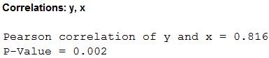
From the MINITAB output, the correlation between the x and y for data set A is 0.816.
Correlation for Data set B:
Software procedure:
Step-by-step procedure to find the correlation between the x and y for data set B by using the MINITAB software:
- Select Stat >Basic Statistics > Correlation.
- In Variables, select x and y.
- Click OK.
Output using the MINITAB software is given below:
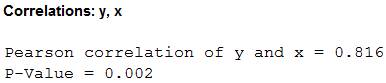
From the MINITAB output, the correlation between the x and y for data set B is 0.816.
Correlation for Data set C:
Software procedure:
Step-by-step procedure to find the correlation between the x and y for data set C by using the MINITAB software:
- Select Stat >Basic Statistics > Correlation.
- In Variables, select x and y.
- Click OK.
Output using the MINITAB software is given below:
From the MINITAB output, the correlation between the x and y for data set C is 0.816.
Correlation for Data set D:
Software procedure:
Step-by-step procedure to find the correlation between the x and y for data set D by using the MINITAB software:
- Select Stat >Basic Statistics > Correlation.
- In Variables, select x and y.
- Click OK.
Output using the MINITAB software is given below:
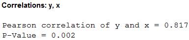
From the MINITAB output, the correlation between the x and y for data set D is 0.817.
Equation of the least-squares line for Data set A:
Software procedure:
Step-by-step procedure to find the equation of the least-squares line by using the MINITAB software:
- Choose Stat > Regression > Regression.
- In Responses, enter the column of y.
- In Predictors, enter the column of x.
- Click OK.
Output using the MINITAB software is given below:
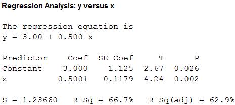
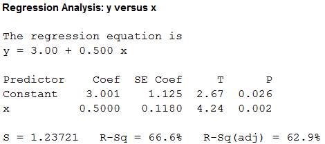
From the MINITAB output, the least-squares line for predicting y from x for data set A is
Equation of the least-squares line for Data set B:
Software procedure:
Step-by-step procedure to find the equation of the least-squares line by using the MINITAB software:
- Choose Stat > Regression > Regression.
- In Responses, enter the column of y.
- In Predictors, enter the column of x.
- Click OK.
Output using the MINITAB software is given below:
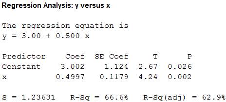
From the MINITAB output, the least-squares line for predicting y from x for data set B is
Equation of the least-squares line for Data set C:
Software procedure:
Step-by-step procedure to find the equation of the least-squares line by using the MINITAB software:
- Choose Stat > Regression > Regression.
- In Responses, enter the column of y.
- In Predictors, enter the column of x.
- Click OK.
Output using the MINITAB software is given below:
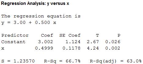
From the MINITAB output, the least-squares line for predicting y from x for data set C is
Equation of the least-squares line for Data set D:
Software procedure:
Step-by-step procedure to find the equation of the least-squares line by using the MINITAB software:
- Choose Stat > Regression > Regression.
- In Responses, enter the column of y.
- In Predictors, enter the column of x.
- Click OK.
Output using the MINITAB software is given below:
From the MINITAB output, the least-squares line for predicting y from x for data set D is
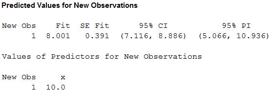
Predicted value for
Software procedure:
Step-by-step procedure to find the predicted value for
- Choose Stat > Regression > Regression.
- In Responses, enter the column of y.
- In Predictors, enter the column of x.
- In option, enter 10 under prediction.
- Click OK.
Output using the MINITAB software is given below:
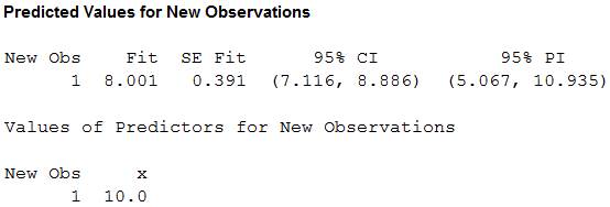
From the MINITAB output, the predicted value for
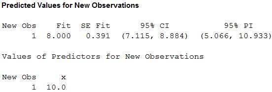
Predicted value for
Software procedure:
Step-by-step procedure to find the predicted value for
- Choose Stat > Regression > Regression.
- In Responses, enter the column of y.
- In Predictors, enter the column of x.
- In option, enter 10 under prediction.
- Click OK.
Output using the MINITAB software is given below:
From the MINITAB output, the predicted value for
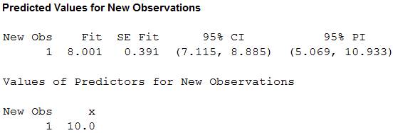
Predicted value for
Software procedure:
Step-by-step procedure to find the predicted value for
- Choose Stat > Regression > Regression.
- In Responses, enter the column of y.
- In Predictors, enter the column of x.
- In option, enter 10 under prediction.
- Click OK.
Output using the MINITAB software is given below:
From the MINITAB output, the predicted value for
From the results, it can be observed that the correlation for all four data sets, the least-squares regression line and the predicted value for
(b)
To construct: The
(b)
Answer to Problem 5.42E
Scatterplot for Data set A:
Output using the MINITAB software is given below:
Scatterplot for Data set B:
Output using the MINITAB software is given below:
Scatterplot for Data set C:
Output using the MINITAB software is given below:
Scatterplot for Data set D:
Output using the MINITAB software is given below:
Explanation of Solution
Calculation:
Scatterplot:
Software procedure:
Step-by-step procedure to construct scatterplot for x and y for all four data sets by using the MINITAB software:
- Choose Graph > Scatter plot.
- Choose With Regression, and then click OK.
- Under Y variables, enter a column of y.
- Under X variables, enter a column of x.
- Click OK.
Observation:
The scatterplot shows that the predicted values are passed through the regression line of the model. Moreover, there is outlier that appears in the x and y directions for the data set A, B, and C. Also, the scatterplot for the data set D shows that the most of the points are plotted around 8.
(c)
To identify: Which of the four cases would you be willing to use the regression line to describe the dependence of y on x.
(c)
Answer to Problem 5.42E
The data set A would use the regression line to describe the dependence of y on x.
Explanation of Solution
From the scatterplots for all data sets, it can be observed that the points for data set A are scattered around the straight line when compared to the other data sets. Hence, the data set A would use the regression line to describe the dependence of y on x.
Want to see more full solutions like this?
Chapter 5 Solutions
Basic Practice of Statistics (Instructor's)


- Client 1 Weight before diet (pounds) Weight after diet (pounds) 128 120 2 131 123 3 140 141 4 178 170 5 121 118 6 136 136 7 118 121 8 136 127 a) Determine the mean change in patient weight from before to after the diet (after – before). What is the 95% confidence interval of this mean difference?arrow_forwardIn order to find probability, you can use this formula in Microsoft Excel: The best way to understand and solve these problems is by first drawing a bell curve and marking key points such as x, the mean, and the areas of interest. Once marked on the bell curve, figure out what calculations are needed to find the area of interest. =NORM.DIST(x, Mean, Standard Dev., TRUE). When the question mentions “greater than” you may have to subtract your answer from 1. When the question mentions “between (two values)”, you need to do separate calculation for both values and then subtract their results to get the answer. 1. Compute the probability of a value between 44.0 and 55.0. (The question requires finding probability value between 44 and 55. Solve it in 3 steps. In the first step, use the above formula and x = 44, calculate probability value. In the second step repeat the first step with the only difference that x=55. In the third step, subtract the answer of the first part from the…arrow_forwardIf a uniform distribution is defined over the interval from 6 to 10, then answer the followings: What is the mean of this uniform distribution? Show that the probability of any value between 6 and 10 is equal to 1.0 Find the probability of a value more than 7. Find the probability of a value between 7 and 9. The closing price of Schnur Sporting Goods Inc. common stock is uniformly distributed between $20 and $30 per share. What is the probability that the stock price will be: More than $27? Less than or equal to $24? The April rainfall in Flagstaff, Arizona, follows a uniform distribution between 0.5 and 3.00 inches. What is the mean amount of rainfall for the month? What is the probability of less than an inch of rain for the month? What is the probability of exactly 1.00 inch of rain? What is the probability of more than 1.50 inches of rain for the month? The best way to solve this problem is begin by creating a chart. Clearly mark the range, identifying the lower and upper…arrow_forward
- Problem 1: The mean hourly pay of an American Airlines flight attendant is normally distributed with a mean of 40 per hour and a standard deviation of 3.00 per hour. What is the probability that the hourly pay of a randomly selected flight attendant is: Between the mean and $45 per hour? More than $45 per hour? Less than $32 per hour? Problem 2: The mean of a normal probability distribution is 400 pounds. The standard deviation is 10 pounds. What is the area between 415 pounds and the mean of 400 pounds? What is the area between the mean and 395 pounds? What is the probability of randomly selecting a value less than 395 pounds? Problem 3: In New York State, the mean salary for high school teachers in 2022 was 81,410 with a standard deviation of 9,500. Only Alaska’s mean salary was higher. Assume New York’s state salaries follow a normal distribution. What percent of New York State high school teachers earn between 70,000 and 75,000? What percent of New York State high school…arrow_forwardPls help asaparrow_forwardSolve the following LP problem using the Extreme Point Theorem: Subject to: Maximize Z-6+4y 2+y≤8 2x + y ≤10 2,y20 Solve it using the graphical method. Guidelines for preparation for the teacher's questions: Understand the basics of Linear Programming (LP) 1. Know how to formulate an LP model. 2. Be able to identify decision variables, objective functions, and constraints. Be comfortable with graphical solutions 3. Know how to plot feasible regions and find extreme points. 4. Understand how constraints affect the solution space. Understand the Extreme Point Theorem 5. Know why solutions always occur at extreme points. 6. Be able to explain how optimization changes with different constraints. Think about real-world implications 7. Consider how removing or modifying constraints affects the solution. 8. Be prepared to explain why LP problems are used in business, economics, and operations research.arrow_forward
- ged the variance for group 1) Different groups of male stalk-eyed flies were raised on different diets: a high nutrient corn diet vs. a low nutrient cotton wool diet. Investigators wanted to see if diet quality influenced eye-stalk length. They obtained the following data: d Diet Sample Mean Eye-stalk Length Variance in Eye-stalk d size, n (mm) Length (mm²) Corn (group 1) 21 2.05 0.0558 Cotton (group 2) 24 1.54 0.0812 =205-1.54-05T a) Construct a 95% confidence interval for the difference in mean eye-stalk length between the two diets (e.g., use group 1 - group 2).arrow_forwardAn article in Business Week discussed the large spread between the federal funds rate and the average credit card rate. The table below is a frequency distribution of the credit card rate charged by the top 100 issuers. Credit Card Rates Credit Card Rate Frequency 18% -23% 19 17% -17.9% 16 16% -16.9% 31 15% -15.9% 26 14% -14.9% Copy Data 8 Step 1 of 2: Calculate the average credit card rate charged by the top 100 issuers based on the frequency distribution. Round your answer to two decimal places.arrow_forwardPlease could you check my answersarrow_forward
- Let Y₁, Y2,, Yy be random variables from an Exponential distribution with unknown mean 0. Let Ô be the maximum likelihood estimates for 0. The probability density function of y; is given by P(Yi; 0) = 0, yi≥ 0. The maximum likelihood estimate is given as follows: Select one: = n Σ19 1 Σ19 n-1 Σ19: n² Σ1arrow_forwardPlease could you help me answer parts d and e. Thanksarrow_forwardWhen fitting the model E[Y] = Bo+B1x1,i + B2x2; to a set of n = 25 observations, the following results were obtained using the general linear model notation: and 25 219 10232 551 XTX = 219 10232 3055 133899 133899 6725688, XTY 7361 337051 (XX)-- 0.1132 -0.0044 -0.00008 -0.0044 0.0027 -0.00004 -0.00008 -0.00004 0.00000129, Construct a multiple linear regression model Yin terms of the explanatory variables 1,i, x2,i- a) What is the value of the least squares estimate of the regression coefficient for 1,+? Give your answer correct to 3 decimal places. B1 b) Given that SSR = 5550, and SST=5784. Calculate the value of the MSg correct to 2 decimal places. c) What is the F statistics for this model correct to 2 decimal places?arrow_forward
 MATLAB: An Introduction with ApplicationsStatisticsISBN:9781119256830Author:Amos GilatPublisher:John Wiley & Sons Inc
 Probability and Statistics for Engineering and th...StatisticsISBN:9781305251809Author:Jay L. DevorePublisher:Cengage Learning
 Statistics for The Behavioral Sciences (MindTap C...StatisticsISBN:9781305504912Author:Frederick J Gravetter, Larry B. WallnauPublisher:Cengage Learning
 Elementary Statistics: Picturing the World (7th E...StatisticsISBN:9780134683416Author:Ron Larson, Betsy FarberPublisher:PEARSON
 The Basic Practice of StatisticsStatisticsISBN:9781319042578Author:David S. Moore, William I. Notz, Michael A. FlignerPublisher:W. H. Freeman
 Introduction to the Practice of StatisticsStatisticsISBN:9781319013387Author:David S. Moore, George P. McCabe, Bruce A. CraigPublisher:W. H. Freeman