
Videos
Determine the roots of
(a)
To calculate: The real roots of the equation
Answer to Problem 4P
Solution: Graphically, the real roots of the equation are approximated as
Explanation of Solution
Given Information: The equation
Formula used: The roots of an equation can be represented graphically by the x-coordinate of the point where the graph intercepts the x-axis.
Calculation:
Use the following MATLAB code to plot the function
Execute the above code to obtain the plot as,
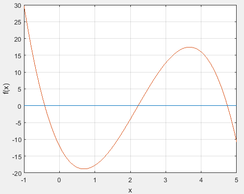
From the plot, the zeros of the equation are approximated as
(b)
To calculate: The root of the equation
Answer to Problem 4P
Solution: The root of the equation is approximated as
Explanation of Solution
Given Information: The function equation is
Initial guesses are,
Formula used: A root of an equation can be obtained using the bisection method as follows:
1. Choose two values of x, say a and b such that
2. Estimate the root by
3. If,
Calculation:
For the function
Thus,
Calculate the first root to be,
Further,
Thus,
Calculate the second root to be:
The approximate error is computed as:
Therefore, the approximate relative percentage error is 100%.
Furthermore,
Thus,
Calculate the third root to be:
The approximate error is computed as:
The approximate error is 33.3%.
Further,
Thus,
Calculate the fourth root to be:
The approximate error is computed as:
The approximate error is 14.28%.
Thus,
Therefore,
Calculate the fifth root to be:
The approximate error is computed as:
The approximate error is 7.69%.
Thus,
Therefore,
Calculate the sixth root to be:
The approximate error is computed as:
The approximate error is 3.7%.
Thus,
Therefore,
Calculate the seventh root to be:
The approximate error is computed as:
The approximate error is 1.89%.
Further,
Thus,
Calculate the eighth root to be:
The approximate error is computed as:
The approximate error is 0.93%.
As,
(c)
To calculate: The root of the equation
Answer to Problem 4P
Solution: The root of the equation can be approximated as
Explanation of Solution
Given Information: The equation
Initial guesses are,
Formula used: A root of an equation can be obtained using the false-position method as follows:
1. Choose two values of x, say a and b such that
2. Estimate the root by
3. If,
Calculation:
For the function
Thus,
Calculate the first root to be,
Now,
Thus,
Calculate the second root to be:
The approximate error is computed as:
The approximate relative percentage error is 24.25%.
Further,
Thus,
Calculate the third root to be:
The approximate error is computed as:
The approximate error is 6.36%.
Now,
Thus,
Calculate the fourth root to be:
The approximate error is computed as:
The approximate error is 1.68%.
Now,
Thus,
Calculate the fifth root would be:
The approximate error is computed as:
The approximate error is 0.45%.
As,
Want to see more full solutions like this?
Chapter 5 Solutions
Numerical Methods For Engineers, 7 Ed
Additional Math Textbook Solutions
University Calculus
University Calculus: Early Transcendentals (4th Edition)
Algebra and Trigonometry (6th Edition)
Mathematics for the Trades: A Guided Approach (11th Edition) (What's New in Trade Math)
Beginning and Intermediate Algebra
Calculus: Early Transcendentals (2nd Edition)


- CORRECT AND DETAILED SOLUTION WITH FBD ONLY. I WILL UPVOTE THANK YOU. CORRECT ANSWER IS ALREADY PROVIDED. I REALLY NEED FBD A concrete wall retains water as shown. Assume that the wall is fixed at the base. Given: H = 3 m, t = 0.5m, Concrete unit weight = 23 kN/m3Unit weight of water = 9.81 kN/m3(Hint: The pressure of water is linearly increasing from the surface to the bottom with intensity 9.81d.)1. Find the maximum compressive stress (MPa) at the base of the wall if the water reaches the top.2. If the maximum compressive stress at the base of the wall is not to exceed 0.40 MPa, what is the maximum allowable depth(m) of the water?3. If the tensile stress at the base is zero, what is the maximum allowable depth (m) of the water?ANSWERS: (1) 1.13 MPa, (2) 2.0 m, (3) 1.20 marrow_forwardCORRECT AND DETAILED SOLUTION WITH FBD ONLY. I WILL UPVOTE THANK YOU. CORRECT ANSWER IS ALREADY PROVIDED. I NEED FBD A short plate is attached to the center of the shaft as shown. The bottom of the shaft is fixed to the ground.Given: a = 75 mm, h = 125 mm, D = 38 mmP1 = 24 kN, P2 = 28 kN1. Calculate the maximum torsional stress in the shaft, in MPa.2. Calculate the maximum flexural stress in the shaft, in MPa.3. Calculate the maximum horizontal shear stress in the shaft, in MPa.ANSWERS: (1) 167.07 MPa; (2) 679.77 MPa; (3) 28.22 MPaarrow_forwardCORRECT AND DETAILED SOLUTION WITH FBD ONLY. I WILL UPVOTE THANK YOU. CORRECT ANSWER IS ALREADY PROVIDED. I REALLY NEED FBD. The roof truss shown carries roof loads, where P = 10 kN. The truss is consisting of circular arcs top andbottom chords with radii R + h and R, respectively.Given: h = 1.2 m, R = 10 m, s = 2 m.Allowable member stresses:Tension = 250 MPaCompression = 180 MPa1. If member KL has square section, determine the minimum dimension (mm).2. If member KL has circular section, determine the minimum diameter (mm).3. If member GH has circular section, determine the minimum diameter (mm).ANSWERS: (1) 31.73 mm; (2) 35.81 mm; (3) 18.49 mmarrow_forward
- PROBLEM 3.23 3.23 Under normal operating condi- tions a motor exerts a torque of magnitude TF at F. The shafts are made of a steel for which the allowable shearing stress is 82 MPa and have diameters of dCDE=24 mm and dFGH = 20 mm. Knowing that rp = 165 mm and rg114 mm, deter- mine the largest torque TF which may be exerted at F. TF F rG- rp B CH TE Earrow_forward1. (16%) (a) If a ductile material fails under pure torsion, please explain the failure mode and describe the observed plane of failure. (b) Suppose a prismatic beam is subjected to equal and opposite couples as shown in Fig. 1. Please sketch the deformation and the stress distribution of the cross section. M M Fig. 1 (c) Describe the definition of the neutral axis. (d) Describe the definition of the modular ratio.arrow_forwardusing the theorem of three moments, find all the moments, I only need concise calculations with minimal explanations. The correct answers are provided at the bottomarrow_forward
 Elements Of ElectromagneticsMechanical EngineeringISBN:9780190698614Author:Sadiku, Matthew N. O.Publisher:Oxford University Press
 Mechanics of Materials (10th Edition)Mechanical EngineeringISBN:9780134319650Author:Russell C. HibbelerPublisher:PEARSON
 Thermodynamics: An Engineering ApproachMechanical EngineeringISBN:9781259822674Author:Yunus A. Cengel Dr., Michael A. BolesPublisher:McGraw-Hill Education
 Control Systems EngineeringMechanical EngineeringISBN:9781118170519Author:Norman S. NisePublisher:WILEY
 Mechanics of Materials (MindTap Course List)Mechanical EngineeringISBN:9781337093347Author:Barry J. Goodno, James M. GerePublisher:Cengage Learning
 Engineering Mechanics: StaticsMechanical EngineeringISBN:9781118807330Author:James L. Meriam, L. G. Kraige, J. N. BoltonPublisher:WILEY