
a.
To calculate: Future value of $1,000 after 5 years at 10% annual interest rate.
Introduction:
a.
Explanation of Solution
Calculation in spreadsheet by “FV” formula,
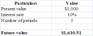
Table (1)
Steps required to calculate
- Select ‘Formulas’ option from Menu Bar of Excel sheet.
- Select insert Function that is (fx).
- Choose category of Financial.
- Then select “FV” and then press OK.
- A window will pop up.
- Input data in the required field.
- Final answer will be shown by the formula that is $1,610.50.
Future value of $1,000 is $1,610.51.
b.
To calculate: Investments future value at 0%,5% and 20% rate after 0,1,2,3,4 and 5 years.
Introduction:
Time Value of Money: It is a vital concept to the investors, as it suggests them the money they are having today is worth more than the value promised in the future.
b.
Explanation of Solution
Calculation spreadsheet by “FV” formula,
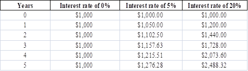
Table (2)
Steps required to calculate present value by using “FV” function in excel are given,
- Select ‘Formulas’ option from Menu Bar of Excel sheet.
- Select insert Function that is (fx).
- Choose category of Financial.
- Then select “FV” and then press OK.
- A window will pop up.
- Input data in required field.
Investment future values are different for the different years with 0%, 5% and 20% interest rate.
c.
To calculate: Present value due of $1,000 in 5 years at the discount rate of 10%.
Introduction:
Time Value of Money: It is a vital concept to the investors, as it suggests them the money they are having today is worth more than the value promised in the future.
c.
Explanation of Solution
Calculation in spreadsheet by “PV” formula,
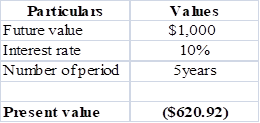
Table (3)
Steps required to calculate present value by using “PV” function in excel are given,
- Select ‘Formulas’ option from Menu Bar of Excel sheet.
- Select insert Function that is (fx).
- Choose category of Financial.
- Then select “PV” and then press OK.
- A window will pop up.
- Input data in the required field.
- Final answer will be shown by the formula that is $620.92.
Present value of $1,000 is $620.92 at 10 % discount rate.
d.
To calculate:
Introduction:
Time Value of Money: It is a vital concept to the investors, as it suggests them the money they are having today is worth more than the value promised in the future.
d.
Explanation of Solution
Calculationin spreadsheet by “RATE” formula,
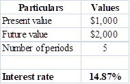
Table (4)
Steps required to calculate present value by using “RATE” function in excel are given,
- Select ‘Formulas’ option from Menu Bar of Excel sheet.
- Select insert Function that is (fx).
- Choose category of Financial.
- Then select “RATE” and then press OK.
- A window will pop up.
- Input data in the required field.
- Final answer will be shown by the formula that is 14.87%
The rate of return is14.87%.
e.
To calculate: Time taken by 36.5 million populations to double with annual growth rate of 2%
Introduction:
Time Value of Money: It is a vital concept to the investors, as it suggests them the money they are having today is worth more than the value promised in the future.
e.
Explanation of Solution
Calculation is solved in spreadsheet by “NPER” formula
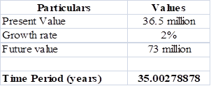
Table (5)
Steps required to calculate present value by using “NPER” function in excel are given,
- Select ‘Formulas’ option from Menu Bar of excel sheet.
- Select insert Function that is (fx).
- Choose category of Financial.
- Then select “NPER” and then press OK.
- A window will pop up.
- Input data in the required field.
- Final answer will be shown by the formula that is 35 years.
Conclusion:
It will take 35 years to double the population from 36.5 million to 73 million.
f.
To calculate: Present and future value of
Introduction:
Time Value of Money: It is a vital concept to the investors, as it suggests them the money they are having today is worth more than the value promised in the future.
f.
Explanation of Solution
Calculation in spreadsheet by “PV” formula,
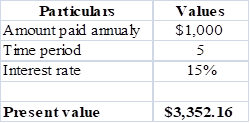
Table (6)
Steps required to calculate present value by using “PV” function in excel are given,
- Select ‘Formulas’ option from Menu Bar of Excel sheet.
- Select insert Function that is (fx).
- Choose category of Financial.
- Then select “PV” and then press OK.
- A window will pop up.
- Input data in the required field.
- Final answer will be shown by the formula that is $3,352.16.
So, the present value is $3,352.16.
Calculation of future value of
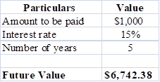
Table (7)
Steps required to calculate present value by using “FV” function in excel are given,
- Select ‘Formulas’ option from Menu Bar of Excel sheet.
- Select insert Function that is (fx).
- Choose category of Financial.
- Then select “FV” and then press OK.
- A window will pop up.
- Input data in the required field.
- Final answer will be shown by the formula that is $6,742.38.
So the future value is $6,742.38.
Present value is $3,352.16 and future value is $6,742.38 of
g.
To calculate: Present and future value of part ‘f’ if the
Introduction:
Time Value of Money: It is a vital concept to the investors, as it suggests them the money they are having today is worth more than the value promised in the future.
g.
Explanation of Solution
Calculation in spreadsheet by “PV” function,
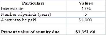
Table (8)
Steps required to calculate present value by using “PV” function in excel are given,
- Select ‘Formulas’ option from Menu Bar of Excel sheet.
- Select insert Function that is (fx).
- Choose category of Financial.
- Then select “PV” and then press OK.
- A window will pop up.
- Input data in the required field.
- Final answer will be shown by the formula that is $3,351.66.
Present value of
Future value of annuity in spreadsheet by “FV” function,
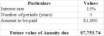
Table (9)
Steps required to calculate present value by using “FV” function in excel are given,
- Select ‘Formulas’ option from Menu Bar of Excel sheet.
- Select insert Function that is (fx).
- Choose category of Financial.
- Then select “FV” and then press OK.
- A window will pop up.
- Input data in the required field.
- Final answer will be shown by the formula that is $7,753.74
Future value of annuity due is $7,753.74.
Present value of
h.
To calculate: Present and future value for $1,000, due in 5 years with 10% semiannual compounding.
Introduction:
Time Value of Money: It is a vital concept to the investors, as it suggests them the money they are having today is worth more than the value promised in the future.
h.
Explanation of Solution
Calculation in spreadsheet by “PV” formula,
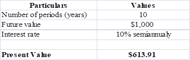
Table (10)
Steps required to calculate present value by using “PV” function in excel are given,
- Select ‘Formulas’ option from Menu Bar of Excel sheet.
- Select insert Function that is (fx).
- Choose category of Financial.
- Then select “PV” and then press OK.
- A window will pop up.
- Input data in the required field.
- Final answer will be shown by the formula that is $613.91.
Present value is $613.91.
Calculation in spreadsheet by “FV” formula,
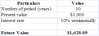
Table (11)
Steps required to calculate present value by using “FV” function in excel are given,
- Select ‘Formulas’ option from Menu Bar of Excel sheet.
- Select insert Function that is (fx).
- Choose category of Financial.
- Then select “FV” and then press OK.
- A window will pop up.
- Input data in the required field.
- Final answer will be shown by the formula that is $1,628.89.
Future value of
Present andfuture value for $1,000, due in 5 years with 10% semiannual compoundingwill be $613.91 and $1,628.89, respectively.
i.
To calculate: Annual payments for an ordinary
Introduction:
Time Value of Money: It is a vital concept to the investors, as it suggests them the money they are having today is worth more than the value promised in the future.
i.
Explanation of Solution
Calculation in spreadsheet by “PMT” formula,
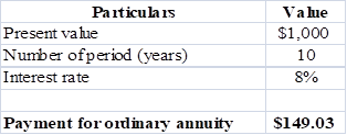
Table (12)
Steps required to calculate present value by using “PMT” function in excel are given,
- Select ‘Formulas’ option from Menu Bar of Excel sheet.
- Select insert Function that is (fx).
- Choose category of Financial.
- Then select “PMT” and then press OK.
- A window will pop up.
- Input data in the required field.
- Final answer will be shown by the formula that is $1,628.89.
Payment of ordinary
Calculation in spreadsheet by “PMT” formula,
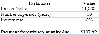
Table (13)
Steps required to calculate present value by using “PMT” function in excel are given,
- Select ‘Formulas’ option from Menu Bar of Excel sheet.
- Select insert Function that is (fx).
- Choose category of Financial.
- Then select “PMT” and then press OK.
- A window will pop up.
- Input data in the required field.
- Final answer will be shown by the formula that is $1,628.89.
Payment of ordinary annuity due is $137.99.
Annual payments are$149.03 for an ordinary
j.
To calculate: Present value and future value of an investment that pays 8% annually and makes the year end payments of $100, $200,$300.
j.
Explanation of Solution
Calculation in spreadsheet by “
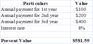
Table (14)
Steps required to calculate present value by using “NPV” function in excel are given,
- Select ‘Formulas’ option from Menu Bar of Excel sheet.
- Select insert Function that is (fx).
- Choose category of Financial.
- Then select “NPV” and then press OK.
- A window will pop up.
- Input data in the required field.
- Final answer will be shown by the formula that is $581.59.
Present value is $581.59.
Calculation in spreadsheet by “FV” formula,
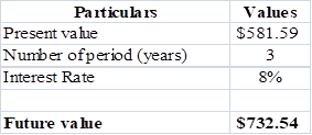
Table (15)
Steps required to calculate present value by using “FV” function in excel are given,
- Select ‘Formulas’ option from Menu Bar of Excel sheet.
- Select insert Function that is (fx).
- Choose category of Financial.
- Then select “FV” and then press OK.
- A window will pop up.
- Input data in the required field.
- Final answer will be shown by the formula that is $732.54.
Future value is $732.54.
Present value is $581.89 while future value is $732.54.
k.1.
To calculate: Effective annual rate each bank pays and the future value of $5,000 at the end of 1 and 2 year.
k.1.
Explanation of Solution
Given for Bank A,
Nominal interest rate is 5%.
Compounding is annual.
Formula to calculate effective annual rate is,
Where,
- EFF is the effective annual rate.
- INOM is the nominal interest rate.
- M is the compounding period.
Substitute 5% for INOM and 1 for M.
So, effective annual rate for Bank A is 5%.
Given for Bank B,
Nominal interest rate is 5%.
Compounding is semiannual.
Formula to calculate effective annual rate is,
Where,
- EFF is the effective annual rate.
- INOM is the nominal interest rate.
- M is the compounding period.
Substitute 5% for INOM and 2 for M.
So,effective annual rate for Bank B is 5.06%.
Given for Bank C,
Nominal interest rate is 5%.
Compounding is quarterly.
Formula to calculate effective annual rate is,
Where,
- EFF is the effective annual rate.
- INOM is the nominal interest rate.
- M is the compounding period.
Substitute 5% for INOM and 4 for M.
So, effective annual rate for Bank C is 5.09%.
Given for Bank D,
Nominal interest rate is 5%.
Compounding ismonthly.
Formula to calculate effective annual rate is,
Where,
- EFF is the effective annual rate.
- INOM is the nominal interest rate.
- M is the compounding period.
Substitute 5% for INOM and 12 for M.
So, effective annual rate for Bank D is 5.11%.
Given for Bank E,
Nominal interest rate is 5%.
Compounding is daily.
Formula to calculate effective annual rate is,
Where,
- EFF is the effective annual rate.
- INOM is the nominal interest rate.
- M is the compounding period.
Substitute 5% for INOM and 365 for M.
So, effective annual rate for Bank E is 5.12%.
Calculation of future value in spreadsheet by “FV” formula,
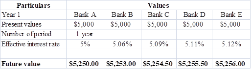
Table (16)
Steps required to calculate present value by using “FV” function in excel are given,
- Select ‘Formulas’ option from Menu Bar of Excel sheet.
- Select insert Function that is (fx).
- Choose category of Financial.
- Then select “FV” and then press OK.
- A window will pop up.
- Input data in the required field.
So, the future value at different effective rate after a year are $5, 250, $5,253,$5,254.50, $5,255.50 and $5,256.
Calculation of future value in spreadsheet by “FV” formula,
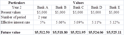
Table (17)
Steps required to calculate present value by using “FV” function in excel are given,
- Select ‘Formulas’ option from Menu Bar of Excel sheet.
- Select insert Function that is (fx).
- Choose category of Financial.
- Then select “FV” and then press OK.
- A window will pop up.
- Input data in the required field.
So, the future value at different effective rate after a year are $5, 512, $5,518.80, $5,521.95, $5,524.06 and $5,525.11.
Each bank pays different effective rate as there compounding is different, the rates are5% for bank A, 5.06% Bank B, 5.09% Bank C, 5.11% Bank D, 5.12% Bank E, also the future values also change on the basis of their number of periods.
2.
To explain: If banks are insured by the government and are equally risky, will they be equally able to attract funds and at what nominal rate all banks provide equal effective rate as Bank A.
2.
Answer to Problem 41SP
No, it is not possible for the banks to equally attract funds.
The nominal rate which causes same effective rate for all banks are,
| Particulars | A | B | C | D | E |
| Nominalrate | 5% | 5.06% | 5.09% | 5.11% | 5.12% |
Table (18)
Explanation of Solution
- Bank will not be equally able to attract funds because of compounding, as people prefer to invest in that bank which have more frequent compounding in comparison to the bank which have lesser frequent compounding.
- Nominal rate is opposite of the effective rate which is calculated in part ‘1’. The nominal rate indicated in above table will cause same effective rate for all banks as it is for A bank.
Due to frequent compounding, banks will not be able to equally attract funds and the nominal rate will be 5% for Bank A, 5.06% Bank B, 5.09% Bank C, 5.11% Bank D, 5.12% Bank E.
3.
To calculate: Present value of amount to get $5,000 after 1 year.
3.
Explanation of Solution
Calculation of payment to be made in spreadsheet by “PMT” formula,
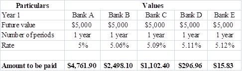
Table (19)
Steps required to calculate present value by using “PMT” function in excel are given,
- Select ‘Formulas’ option from Menu Bar of Excel sheet.
- Select insert Function that is (fx).
- Choose category of Financial.
- Then select “PMT” and then press OK.
- A window will pop up.
- Input data in the required field.
So, the amounts to be paid are$4,761.90,$2498.10,$1,102.40,$296.96 and $15.83.
4.
To explain: If all banks are providing a same effective interest rate would rational investor be indifferent between the banks.
4.
Answer to Problem 41SP
Yes, a rational investor would be indifferent between the banks.
Explanation of Solution
Rational investor chooses the bank which will provide him better return so he would be indifferent, if all the banks are giving same effective rate because he chooses the bank which will have more frequent compounding than others.
A bank offers frequent compounding is able to attract more number of customers than others.
To prepare: Amortization schedule to show annual payments, interest payments, principal payments, and beginning and ending loan balances.
Amortization:
Amotization means to write off or pay the debt over the priod of time it can be for loan or intangible assets. Its main purpose is to get cost recovery. Example of amortization is ,an automobile company that spent $20 million dollars on a design patent with a useful life of 20 years. The amortization value for that company will be $1 million each year.
Explanation of Solution
Calculation of annual installment is done by using “PMT” formula in spreadsheet at the amortization schedule.
Amortization schedule is prepared below,
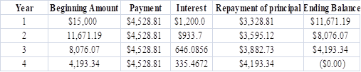
Table (20)
Steps required to calculate present value by using “PMT” function in excel are given,
- Select ‘Formulas’ option from Menu Bar of Excel sheet.
- Select insert Function that is (fx).
- Choose category of Financial.
- Then select “PMT” and then press OK.
- A window will pop up.
- Input data in the required field.
Amortization schedule represents annual payments, interest payments, principal payments, and beginning and ending loan balances.
Want to see more full solutions like this?
Chapter 5 Solutions
Fundamentals of Financial Management, Concise Edition

- Delta Corporation has the following capital structure: Cost Weighted (after-tax) Weights Cost Debt 8.1% 35% 2.84% Preferred stock (Kp) 9.6 5 .48 Common equity (Ke) (retained earnings) 10.1 60 6.06 Weighted average cost of capital (Ka) 9.38% a. If the firm has $18 million in retained earnings, at what size capital structure will the firm run out of retained earnings? b. The 8.1 percent cost of…arrow_forwardDillon Enterprises has the following capDillon Enterprises has the following capital structure. Debt ........................ 40% Common equity ....... 60 The after-tax cost of debt is 6 percent, and the cost of common equity (in the form of retained earnings) is 13 percent. What is the firm’s weighted average cost of capital? a. An outside consultant has suggested that because debt is cheaper than equity, the firm should switch to a capital structure that is 50 percent debt and 50 percent equity. Under this new and more debt-oriented arrangement, the after-tax cost of debt is 7 percent, and the cost of common equity (in the form of retained earnings) is 15 percent. Recalculate the firm’s weighted average cost of capital. b. Which plan is optimal in terms of minimizing the weighted average cost of capital?arrow_forwardCompute Ke and Kn under the following circumstances: a. D1= $5, P0=$70, g=8%, F=$7 b. D1=$0.22, P0=$28, g=7%, F=2.50 c. E1 (earnings at the end of period one) = $7, payout ratio equals 40 percent, P0= $30, g=6%, F=$2,20. Note: D1 is the earnings times the payout rate. d. D0 (dividend at the beginning of the first period) = $6, growth rate for dividends and earnings (g)=7%, P0=$60, F=$3. You will need to calculate D1 (the dividend after the first period).arrow_forward
- Terrier Company is in a 45 percent tax bracket and has a bond outstanding that yields 11 percent to maturity. a. What is Terrier's after-tax cost of debt? b. Assume that the yield on the bond goes down by 1 percentage point, and due to tax reform, the corporate tax falls to 30 percent. What is Terrier's new aftertax cost of debt? c. Has the after-tax cost of debt gone up or down from part a to part b? Explain why.arrow_forwardThe Squeaks Cat Rescue, which is tax-exempt, issued debt last year at 9 percent to help finance a new animal shelter in Rocklin. a. If the rescue borrowed money this year, what would the after-tax cost of debt be, based on its cost last year and the 25 percent increase? b. If the receipts of the rescue were found to be taxable by the IRS (at a rate of 25 percent because of involvement in political activities), what would the after-tax cost of debt be?arrow_forwardNo chatgptPlease don't answer i will give unhelpful all expert giving wrong answer he is giving answer with using incorrect values.arrow_forward
- Please don't answer i will give unhelpful all expert giving wrong answer he is giving answer with incorrect data.arrow_forward4. On August 20, Mr. and Mrs. Cleaver decided to buy a property from Mr. and Mrs. Ward for $105,000. On August 30, Mr. and Mrs. Cleaver obtained a loan commitment from OKAY National Bank for an $84,000 conventional loan at 5 percent for 30 years. The lender informs Mr. and Mrs. Cleaver that a $2,100 loan origination fee will be required to obtain the loan. The loan closing is to take place September 22. In addition, escrow accounts will be required for all prorated property taxes and hazard insurance; however, no mortgage insurance is necessary. The buyer will also pay a full year's premium for hazard insurance to Rock of Gibraltar Insurance Company. A breakdown of expected settlement costs, provided by OKAY National Bank when Mr. and Mrs. Cleaver inspect the uniform settlement statement as required under RESPA on September 21, is as follows: I. Transactions between buyer-borrower and third parties: a. Recording fees--mortgage b. Real estate transfer tax c. Recording fees/document…arrow_forwardHello tutor give correct answerarrow_forward
 Essentials Of InvestmentsFinanceISBN:9781260013924Author:Bodie, Zvi, Kane, Alex, MARCUS, Alan J.Publisher:Mcgraw-hill Education,

 Foundations Of FinanceFinanceISBN:9780134897264Author:KEOWN, Arthur J., Martin, John D., PETTY, J. WilliamPublisher:Pearson,
 Fundamentals of Financial Management (MindTap Cou...FinanceISBN:9781337395250Author:Eugene F. Brigham, Joel F. HoustonPublisher:Cengage Learning
 Corporate Finance (The Mcgraw-hill/Irwin Series i...FinanceISBN:9780077861759Author:Stephen A. Ross Franco Modigliani Professor of Financial Economics Professor, Randolph W Westerfield Robert R. Dockson Deans Chair in Bus. Admin., Jeffrey Jaffe, Bradford D Jordan ProfessorPublisher:McGraw-Hill Education