Concept explainers
Videos
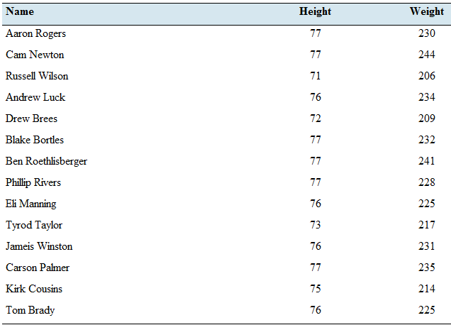
Pass the ball: The following table lists the heights (inches) and weights (pounds) of 14 National Football League quarterbacks in the 2016 season.
- Compute the least-squares regression line for predicting weight from height.
- Is it possible to interpret the y-intercept? Explain.
- If two quarterbacks differ in height by two inches: by how much would you predict their weights to differ?
- Predict the of a quarterback who is 74.5 inches tall.
- Kirk Cousins is 75 inches tall and weighs 214 pounds. Does he weigh more or less than the weight predicted by the least-squares regression line?
a.
To find: The least-square regression line for the given data set.
Answer to Problem 23E
The least square regression line of the given data set is,
Explanation of Solution
Following table with the heights and the weights of the national football quarterbacks in the season
| Name | Height | Weight |
| Aaron Rogers | 77 | 230 |
| Cam Newton | 77 | 244 |
| Russell Wilson | 71 | 206 |
| Andrew Luck | 76 | 234 |
| Drew Brees | 72 | 209 |
| Blake Bortles | 77 | 232 |
| Ben Roethlisberger | 77 | 241 |
| Philip Rivers | 77 | 228 |
| Eli Manning | 76 | 225 |
| Tyrod Taylor | 73 | 217 |
| Jamies Winston | 76 | 231 |
| Carson Palmer | 77 | 235 |
| Kirk Cousins | 75 | 214 |
| Tom Brady | 76 | 225 |
Calculation:
The least-square regression is given by the formula,
Where
The correlation coefficient is given by the formula,
Let
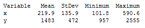
The correlation coefficient can be obtained by the following table.
Hence, the correlation coefficient is,
Then, the coefficient
Therefore,
Conclusion:
The least square regression line is found to be,
b.
To explain:The possibility to interpret the
Answer to Problem 23E
The
Explanation of Solution
The least-square regression line has been computed as
Considering the
The
Conclusion:
There is no chance to a weight be a negative value. Therefore, this
c.
To calculate:The difference in the weight of two players when their heights differ by two inches.
Answer to Problem 23E
The difference of weight is found to be
Explanation of Solution
The least-square regression line has been computed as
Calculation:
Let the height of the shorter payer be
Also, the weight of the taller player should be,
Simplifying the obtained weight,
Therefore, the difference of two weights should be,
Interpretation:
As the calculation above, the weight difference for two inches change in the height is found to be
d.
To find:The predicted weight of a player whose height is
Answer to Problem 23E
The weight of a player whose height is
Explanation of Solution
Calculation:
By the computed least-square regression line, we can calculate the predictions for the weights of the players by substituting their heights into the formula.
Here, the height is said to be
Conclusion:
The weight of a player whose height is
e.
To find:Whether theactual weight of this player is greater than the predicted weight or not.
Answer to Problem 23E
The player weighs less than the predicted weight.
Explanation of Solution
The player is
Calculation:
When the height is said to be
The predicted weight is found to be
Conclusion:
Since
Want to see more full solutions like this?
Chapter 4 Solutions
Loose Leaf Version For Elementary Statistics


- You may need to use the appropriate appendix table or technology to answer this question. You are given the following information obtained from a random sample of 4 observations. 24 48 31 57 You want to determine whether or not the mean of the population from which this sample was taken is significantly different from 49. (Assume the population is normally distributed.) (a) State the null and the alternative hypotheses. (Enter != for ≠ as needed.) H0: Ha: (b) Determine the test statistic. (Round your answer to three decimal places.) (c) Determine the p-value, and at the 5% level of significance, test to determine whether or not the mean of the population is significantly different from 49. Find the p-value. (Round your answer to four decimal places.) p-value = State your conclusion. Reject H0. There is insufficient evidence to conclude that the mean of the population is different from 49.Do not reject H0. There is sufficient evidence to conclude that the…arrow_forward65% of all violent felons in the prison system are repeat offenders. If 43 violent felons are randomly selected, find the probability that a. Exactly 28 of them are repeat offenders. b. At most 28 of them are repeat offenders. c. At least 28 of them are repeat offenders. d. Between 22 and 26 (including 22 and 26) of them are repeat offenders.arrow_forward08:34 ◄ Classroom 07:59 Probs. 5-32/33 D ا. 89 5-34. Determine the horizontal and vertical components of reaction at the pin A and the normal force at the smooth peg B on the member. A 0,4 m 0.4 m Prob. 5-34 F=600 N fr th ar 0. 163586 5-37. The wooden plank resting between the buildings deflects slightly when it supports the 50-kg boy. This deflection causes a triangular distribution of load at its ends. having maximum intensities of w, and wg. Determine w and wg. each measured in N/m. when the boy is standing 3 m from one end as shown. Neglect the mass of the plank. 0.45 m 3 marrow_forward
- Examine the Variables: Carefully review and note the names of all variables in the dataset. Examples of these variables include: Mileage (mpg) Number of Cylinders (cyl) Displacement (disp) Horsepower (hp) Research: Google to understand these variables. Statistical Analysis: Select mpg variable, and perform the following statistical tests. Once you are done with these tests using mpg variable, repeat the same with hp Mean Median First Quartile (Q1) Second Quartile (Q2) Third Quartile (Q3) Fourth Quartile (Q4) 10th Percentile 70th Percentile Skewness Kurtosis Document Your Results: In RStudio: Before running each statistical test, provide a heading in the format shown at the bottom. “# Mean of mileage – Your name’s command” In Microsoft Word: Once you've completed all tests, take a screenshot of your results in RStudio and paste it into a Microsoft Word document. Make sure that snapshots are very clear. You will need multiple snapshots. Also transfer these results to the…arrow_forwardExamine the Variables: Carefully review and note the names of all variables in the dataset. Examples of these variables include: Mileage (mpg) Number of Cylinders (cyl) Displacement (disp) Horsepower (hp) Research: Google to understand these variables. Statistical Analysis: Select mpg variable, and perform the following statistical tests. Once you are done with these tests using mpg variable, repeat the same with hp Mean Median First Quartile (Q1) Second Quartile (Q2) Third Quartile (Q3) Fourth Quartile (Q4) 10th Percentile 70th Percentile Skewness Kurtosis Document Your Results: In RStudio: Before running each statistical test, provide a heading in the format shown at the bottom. “# Mean of mileage – Your name’s command” In Microsoft Word: Once you've completed all tests, take a screenshot of your results in RStudio and paste it into a Microsoft Word document. Make sure that snapshots are very clear. You will need multiple snapshots. Also transfer these results to the…arrow_forwardExamine the Variables: Carefully review and note the names of all variables in the dataset. Examples of these variables include: Mileage (mpg) Number of Cylinders (cyl) Displacement (disp) Horsepower (hp) Research: Google to understand these variables. Statistical Analysis: Select mpg variable, and perform the following statistical tests. Once you are done with these tests using mpg variable, repeat the same with hp Mean Median First Quartile (Q1) Second Quartile (Q2) Third Quartile (Q3) Fourth Quartile (Q4) 10th Percentile 70th Percentile Skewness Kurtosis Document Your Results: In RStudio: Before running each statistical test, provide a heading in the format shown at the bottom. “# Mean of mileage – Your name’s command” In Microsoft Word: Once you've completed all tests, take a screenshot of your results in RStudio and paste it into a Microsoft Word document. Make sure that snapshots are very clear. You will need multiple snapshots. Also transfer these results to the…arrow_forward
- 2 (VaR and ES) Suppose X1 are independent. Prove that ~ Unif[-0.5, 0.5] and X2 VaRa (X1X2) < VaRa(X1) + VaRa (X2). ~ Unif[-0.5, 0.5]arrow_forward8 (Correlation and Diversification) Assume we have two stocks, A and B, show that a particular combination of the two stocks produce a risk-free portfolio when the correlation between the return of A and B is -1.arrow_forward9 (Portfolio allocation) Suppose R₁ and R2 are returns of 2 assets and with expected return and variance respectively r₁ and 72 and variance-covariance σ2, 0%½ and σ12. Find −∞ ≤ w ≤ ∞ such that the portfolio wR₁ + (1 - w) R₂ has the smallest risk.arrow_forward
- 7 (Multivariate random variable) Suppose X, €1, €2, €3 are IID N(0, 1) and Y2 Y₁ = 0.2 0.8X + €1, Y₂ = 0.3 +0.7X+ €2, Y3 = 0.2 + 0.9X + €3. = (In models like this, X is called the common factors of Y₁, Y₂, Y3.) Y = (Y1, Y2, Y3). (a) Find E(Y) and cov(Y). (b) What can you observe from cov(Y). Writearrow_forward1 (VaR and ES) Suppose X ~ f(x) with 1+x, if 0> x > −1 f(x) = 1−x if 1 x > 0 Find VaRo.05 (X) and ES0.05 (X).arrow_forwardJoy is making Christmas gifts. She has 6 1/12 feet of yarn and will need 4 1/4 to complete our project. How much yarn will she have left over compute this solution in two different ways arrow_forward
 Glencoe Algebra 1, Student Edition, 9780079039897...AlgebraISBN:9780079039897Author:CarterPublisher:McGraw Hill
 Big Ideas Math A Bridge To Success Algebra 1: Stu...AlgebraISBN:9781680331141Author:HOUGHTON MIFFLIN HARCOURTPublisher:Houghton Mifflin Harcourt
 Holt Mcdougal Larson Pre-algebra: Student Edition...AlgebraISBN:9780547587776Author:HOLT MCDOUGALPublisher:HOLT MCDOUGAL
 Functions and Change: A Modeling Approach to Coll...AlgebraISBN:9781337111348Author:Bruce Crauder, Benny Evans, Alan NoellPublisher:Cengage Learning