
Concept explainers
Videos
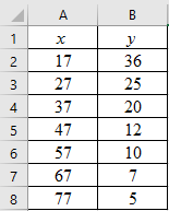
Auto Accidents: Age Data for this problem are based on information taken from The Wall Street Journal. Let x be the age in years of a licensed automobile driver. Let y be the percentage of all fatal accidents (for a given age) due to speeding. For example, the first data pair indicates that 36% of all fatal accidents involving 17-year-olds are due to speeding.
| x | 17 | 27 | 37 | 47 | 57 | 67 | 77 |
| y | 36 | 25 | 20 | 12 | 10 | 7 | 5 |
Complete parts (a) through (e), given
(f) Predict the percentage of all fatal accidents due to speeding for 25-year-olds.
(a)
To graph: The scatter diagram for age in years of a licensed automobile driver (x) and percentage of all fatal accidents (y).
Explanation of Solution
Given: The data which consists of variables, ‘age of a licensed automobile driver (in years)’ and ‘the percentage of all fatal accidents (for a given age)’ due to speeding, represented by x and y respectively, is provided.
Graph:
Follow the steps given below in Excel to obtain the scatter diagram of the data.
Step 1: Enter the data into Excel sheet. The screenshot is given below.
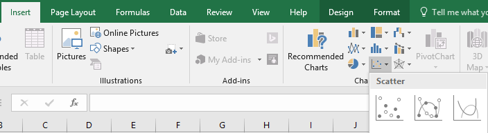
Step 2: Select the data and click on ‘Insert’. Go to charts and select the chart type ‘Scatter’.
Step 3: Select the first plot and then click ‘add chart element’ provided in the left corner of the menu bar. Insert the ‘Axis titles’ and ‘Chart title’. The scatter plot for the provided data is shown below:
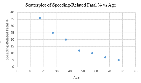
Interpretation: The scatterplot shows that, there is a negative correlation between the age of a licensed automobile drivers and the speeding- related fatal percentage. So, as the age increases, the fatal percentage related to speeding decreases and vice versa.
(b)
To test: Whether the provided values of
Answer to Problem 11P
Solution: The provided values, that is,
Explanation of Solution
Given: The provided values are:
Calculation:
To compute
| 17 | 36 | 289 | 1296 | 612 |
| 27 | 25 | 729 | 625 | 675 |
| 37 | 20 | 1369 | 400 | 740 |
| 47 | 12 | 2209 | 144 | 564 |
| 57 | 10 | 3249 | 100 | 570 |
| 67 | 7 | 4489 | 49 | 469 |
| 77 | 5 | 5929 | 25 | 385 |
Now, the value of
Substituting the values in the above formula. Thus:
Thus, the value of
Conclusion: The provided values,
(c)
To find: The values of
Answer to Problem 11P
Solution: The calculated values are,
Explanation of Solution
Given: The provided values are,
Calculation:
The value of
The value of
The value of
The value of
Therefore, the values are,
The general formula for the least-squares line is,
Here, a is the y-intercept and b is the slope.
Substitute the values of a and b in the general equation, to get the least-squares line of the data. That is,
Therefore, the least-squares line is
(d)
To graph: The least-squares line on the scatter diagram which passes through the point
Explanation of Solution
Given: The data which consists of variables, ‘age of a licensed automobile driver (in years)’ and ‘the fatal accidents percentage (for a given age) due to speeding’, represented by x and y respectively, is provided.
Graph:
Follow the steps given below in Excel to obtain the scatter diagram of the data.
Step 1: Enter the data into Excel sheet. The screenshot is given below.
Step 2: Select the data and click on ‘Insert’. Go to charts and select the chart type ‘Scatter’.
Step 3: Select the first plot and then click ‘add chart element’ provided in the left corner of the menu bar. Insert the ‘Axis titles’ and ‘Chart title’. The scatter plot for the provided data is shown below:
Step 3: Right click on any data point and select ‘Add Trendline’. In the dialogue box, select ‘linear’ and check ‘Display Equation on Chart’
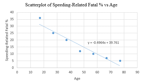
Interpretation: The least-squares line passes through the point
(e)
The value of
Answer to Problem 11P
Solution: The value of
Explanation of Solution
Given: The value of the correlation coefficient (r) is
Calculation: The coefficient of determination
Therefore, the value of
The value of
Further, the proportion of variation in y that is unexplained can be calculated as:
Hence, the percentage of variation in y that is unexplained is 8%.
Interpretation: About 92% of the variation in y (fatal % due to speeding) can be explained by the corresponding variation in x (age) and the least-squares line. The rest 8% of variation remains unexplained.
(f)
To find: The predicted percentage of speeding related fatal accidents
Answer to Problem 11P
Solution: The predicted value is approximately 27.36%.
Explanation of Solution
Given: The least-squares line from part (c) is,
Calculation:
The predicted value
Thus, the value of
Interpretation: The percentage of all fatal accidents due to speeding for 25-years-olds is predicted to be 27.36%.
Want to see more full solutions like this?
Chapter 4 Solutions
Understanding Basic Statistics


- Consider the hypothesis test Ho: = 622 against H₁: 6 > 62. Suppose that the sample sizes are n₁ = 20 and n₂ = 8, and that = 4.5; s=2.3. Use a = 0.01. (a) Test the hypothesis. Round your answers to two decimal places (e.g. 98.76). The test statistic is fo = i The critical value is f = Conclusion: i the null hypothesis at a = 0.01. (b) Construct the confidence interval on 02/022 which can be used to test the hypothesis: (Round your answer to two decimal places (e.g. 98.76).) iarrow_forward2011 listing by carmax of the ages and prices of various corollas in a ceratin regionarrow_forwardس 11/ أ . اذا كانت 1 + x) = 2 x 3 + 2 x 2 + x) هي متعددة حدود محسوبة باستخدام طريقة الفروقات المنتهية (finite differences) من جدول البيانات التالي للدالة (f(x . احسب قيمة . ( 2 درجة ) xi k=0 k=1 k=2 k=3 0 3 1 2 2 2 3 αarrow_forward
- 1. Differentiate between discrete and continuous random variables, providing examples for each type. 2. Consider a discrete random variable representing the number of patients visiting a clinic each day. The probabilities for the number of visits are as follows: 0 visits: P(0) = 0.2 1 visit: P(1) = 0.3 2 visits: P(2) = 0.5 Using this information, calculate the expected value (mean) of the number of patient visits per day. Show all your workings clearly. Rubric to follow Definition of Random variables ( clearly and accurately differentiate between discrete and continuous random variables with appropriate examples for each) Identification of discrete random variable (correctly identifies "number of patient visits" as a discrete random variable and explains reasoning clearly.) Calculation of probabilities (uses the probabilities correctly in the calculation, showing all steps clearly and logically) Expected value calculation (calculate the expected value (mean)…arrow_forwardif the b coloumn of a z table disappeared what would be used to determine b column probabilitiesarrow_forwardConstruct a model of population flow between metropolitan and nonmetropolitan areas of a given country, given that their respective populations in 2015 were 263 million and 45 million. The probabilities are given by the following matrix. (from) (to) metro nonmetro 0.99 0.02 metro 0.01 0.98 nonmetro Predict the population distributions of metropolitan and nonmetropolitan areas for the years 2016 through 2020 (in millions, to four decimal places). (Let x, through x5 represent the years 2016 through 2020, respectively.) x₁ = x2 X3 261.27 46.73 11 259.59 48.41 11 257.96 50.04 11 256.39 51.61 11 tarrow_forward
- If the average price of a new one family home is $246,300 with a standard deviation of $15,000 find the minimum and maximum prices of the houses that a contractor will build to satisfy 88% of the market valuearrow_forward21. ANALYSIS OF LAST DIGITS Heights of statistics students were obtained by the author as part of an experiment conducted for class. The last digits of those heights are listed below. Construct a frequency distribution with 10 classes. Based on the distribution, do the heights appear to be reported or actually measured? Does there appear to be a gap in the frequencies and, if so, how might that gap be explained? What do you know about the accuracy of the results? 3 4 555 0 0 0 0 0 0 0 0 0 1 1 23 3 5 5 5 5 5 5 5 5 5 5 5 5 6 6 8 8 8 9arrow_forwardA side view of a recycling bin lid is diagramed below where two panels come together at a right angle. 45 in 24 in Width? — Given this information, how wide is the recycling bin in inches?arrow_forward
- 1 No. 2 3 4 Binomial Prob. X n P Answer 5 6 4 7 8 9 10 12345678 8 3 4 2 2552 10 0.7 0.233 0.3 0.132 7 0.6 0.290 20 0.02 0.053 150 1000 0.15 0.035 8 7 10 0.7 0.383 11 9 3 5 0.3 0.132 12 10 4 7 0.6 0.290 13 Poisson Probability 14 X lambda Answer 18 4 19 20 21 22 23 9 15 16 17 3 1234567829 3 2 0.180 2 1.5 0.251 12 10 0.095 5 3 0.101 7 4 0.060 3 2 0.180 2 1.5 0.251 24 10 12 10 0.095arrow_forwardstep by step on Microssoft on how to put this in excel and the answers please Find binomial probability if: x = 8, n = 10, p = 0.7 x= 3, n=5, p = 0.3 x = 4, n=7, p = 0.6 Quality Control: A factory produces light bulbs with a 2% defect rate. If a random sample of 20 bulbs is tested, what is the probability that exactly 2 bulbs are defective? (hint: p=2% or 0.02; x =2, n=20; use the same logic for the following problems) Marketing Campaign: A marketing company sends out 1,000 promotional emails. The probability of any email being opened is 0.15. What is the probability that exactly 150 emails will be opened? (hint: total emails or n=1000, x =150) Customer Satisfaction: A survey shows that 70% of customers are satisfied with a new product. Out of 10 randomly selected customers, what is the probability that at least 8 are satisfied? (hint: One of the keyword in this question is “at least 8”, it is not “exactly 8”, the correct formula for this should be = 1- (binom.dist(7, 10, 0.7,…arrow_forwardKate, Luke, Mary and Nancy are sharing a cake. The cake had previously been divided into four slices (s1, s2, s3 and s4). What is an example of fair division of the cake S1 S2 S3 S4 Kate $4.00 $6.00 $6.00 $4.00 Luke $5.30 $5.00 $5.25 $5.45 Mary $4.25 $4.50 $3.50 $3.75 Nancy $6.00 $4.00 $4.00 $6.00arrow_forward
 Glencoe Algebra 1, Student Edition, 9780079039897...AlgebraISBN:9780079039897Author:CarterPublisher:McGraw Hill
 Functions and Change: A Modeling Approach to Coll...AlgebraISBN:9781337111348Author:Bruce Crauder, Benny Evans, Alan NoellPublisher:Cengage Learning
 Big Ideas Math A Bridge To Success Algebra 1: Stu...AlgebraISBN:9781680331141Author:HOUGHTON MIFFLIN HARCOURTPublisher:Houghton Mifflin Harcourt
 Holt Mcdougal Larson Pre-algebra: Student Edition...AlgebraISBN:9780547587776Author:HOLT MCDOUGALPublisher:HOLT MCDOUGAL
 Linear Algebra: A Modern IntroductionAlgebraISBN:9781285463247Author:David PoolePublisher:Cengage Learning