Whether there was a statistically significant difference in the average speeds, the mean speed, standard deviation, 85th percentile speed and percentage of traffic exceeding the posted speed limit of 30 mi/h.
Answer to Problem 9P
Significant reduction
Explanation of Solution
Given:
Significance level of
Formula used:
S is standard deviation
N is number of observations
Spis square root of the pooled variance
S1 and S2 are standard deviations of the populations
T is the test static
Calculation:
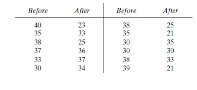
Before an increase in speed enforcement activities:
The speed ranges from 28 to 40 mi/hgiving a speed range of 12. For five classes, the range per class is 2.4mi/h. A frequency distribution table can then be prepared, as shown below, in which the speed classes are listed in column 1 and the mid-values are in column 2. The number of observationsfor each class is listed in column 3, the cumulative percentages of all observations arelisted in column 6.
| 1 | 2 | 3 | 4 | 5 | 6 | 7 |
| Speed class (mi/h) | Class mid-value | Class frequency, | | Percentage of class frequency | Cumulative percentage of class frequency | |
| 28-30 | 29 | 4 | 116 | 13 | 13 | 139.24 |
| 31-33 | 32 | 5 | 160 | 17 | 30 | 42.05 |
| 34-36 | 35 | 12 | 420 | 40 | 70 | 0.12 |
| 37-39 | 38 | 6 | 228 | 20 | 90 | 57.66 |
| 40-42 | 41 | 3 | 123 | 10 | 100 | 111.63 |
| Total | 30 | 1047 | 350.7 |
Determine the arithmetic mean speed:
Determine the standard deviation:
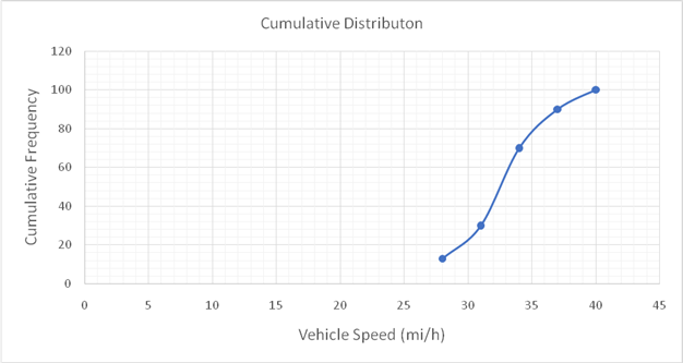
The 85th-percentile speed is obtained from the cumulative frequency distribution curve as 36 mi/h.
The percentage of traffic exceeding the posted speed limit of 30 mi/h is 76 %.
Below given figure shows the cumulative frequency distribution curve for the data given. In this case, the cumulative percentages in column 6 of the above Table are plotted against the upper limit of each corresponding speed class. This curve, therefore, gives the percentage of vehicles that are traveling at or below a given speed.
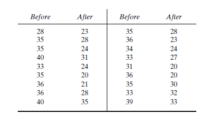
After an increase in speed enforcement activities:
The speed ranges from 20 to 37 mi/h giving a speed range of 17. For six classes, the range per class is 2.83 mi/h. A frequency distribution table can then be prepared, as shown below in which the speed classes are listed in column 1 and the mid-values are in column 2. The number of observations for each class is listed in column 3, the cumulative percentages of all observations are listed in column 6.
| 1 | 2 | 3 | 4 | 5 | 6 | 7 |
| Speed class (mi/h) | Class mid-value | Class frequency, | | Percentage of class frequency | Cumulative percentage of class frequency | |
| 20-22 | 21 | 6 | 126 | 20 | 20 | 253.5 |
| 23-25 | 24 | 8 | 192 | 27 | 47 | 98 |
| 26-28 | 27 | 4 | 108 | 13 | 60 | 1 |
| 29-31 | 30 | 3 | 90 | 10 | 70 | 18.75 |
| 32-34 | 33 | 5 | 165 | 17 | 87 | 151.25 |
| 35-37 | 36 | 4 | 144 | 13 | 100 | 289 |
| Total | 30 | 825 | 811.5 |
Determine the arithmetic mean speed:
Determine the standard deviation:
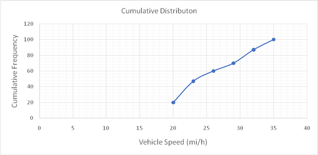
Below given figure shows the cumulative frequency distribution curve for the data given. In this case, the cumulative percentages in column 6 of the above Table are plotted against the upper limit of each corresponding speed class. This curve, therefore, gives the percentage of vehicles that are traveling at or below a given speed.
The 85th-percentile speed is obtained from the cumulative frequency distribution curve as 31.5 mi/h.
The percentage of traffic exceeding the posted speed limit of 30 mi/h is 24 %.
Determine square root of the pooled variance:
Compute test static T:
Determine whether
From Appendix A, theoretical
Since
Conclusion:
The increase in speed enforcement activities has resulted in a significant reduction in the mean speed on the street at a significance level of 0.05. The mean speeds before and after increase in speed enforcement activities are 35.1 and 27.47 mi/h respectively. The standard deviations are 3.5 and 5.3 mi/h respectively. The 85th percentile speeds are 36 mi/h and 31.5 mi/h and percentages of traffic exceeding the posted speed limit of 30 mi/h are 76 % and 24 %.
Want to see more full solutions like this?
Chapter 4 Solutions
Traffic And Highway Engineering

- The head-vs-capacity curves for two centrifugal pumps A and B are shown below: Which of the following is a correct statement at a flow rate of 600 ft3/min? Assuming a pump efficiency of 80%. Head [ft] 50 45 40 35- 30 25 20 15 10 5. 0 0 Pump B Pump A 100 200 300 400 500 600 700 800 900 1000arrow_forwardSolve for reactions and shear and moment diagram (base the answer on the 2nd figure). Hand Calculation 2. Note: Assume bottom left support as roller, bottom right support as pinned 4 kN/m 3 kN/m 8m 4m 2marrow_forwardYour client wants to build a WTP that has a withdraw of 440 MGD. What is the exceedance probability in percentage? Average Monthly Minimum Flow of Record Month (MGD) Jan-73 322 Feb-73 280 Mar-73 335 Apr-73 374 May-73 440 Mar-74 313 Apr-74 375 May-74 560 Jun-74 380 Jul-74 445 Aug-74 323 Sep-74 411 Oct-74 541 Nov-74 510 Jan-75 261 Feb-75 271 May-75 312 Jun-75 314 351 Jul-75 Aug-75 332arrow_forward
- If a second 12.25" pump was added in parallel what would be the NPSHr be while both pumps are running? HEAD (Feet) 250- 200- Pump Series: VSX-VSC 10x12x13-1/2A 1780 RPM 13.5" 60% 70% -75% 80% 83% -85.5%- 150- 12.25" 100- 50 50- 10" 0- 2,000 NPSHr 83%. 80% 300HP- -75% 250HP 200HP 70% 150HP 125HP 100HP NPSHr(ft) 0 4,000 6,000 8,000 Capacity (GPM) 80 90 8arrow_forwardSolve for reactions and shear and moment diagram (base the answer on the 2nd figure) 1. Note: Assume bottom support as pinned 14 kN/m 16 kN 6m 5m 3m- 6marrow_forwardA plant treats 25 MGD at 5°C and pH=7.0. The plant uses ozone before the filter and free chlorine after the filter. The ozone contactor has a t10 of 3 minutes and a residual concentration of 0.3 mg/L. The free chlorine contact basin is 65 ft by 214 ft by 10 ft and a baffle factor of 0.5 and a residual concentration of 1.4 mg/Larrow_forward
- A3-inch diameter water pipe carries a flow rate of 6 gallons per minute. The pipe is 100 feet long and has a gate valve, two 45-degree elbows, and a sudden c factor for the pipe is 0.02 and the minor loss coefficients for the gate valve, elbows, and contraction are 12, 1.5, and 0.5, respectively. Determine the head loss due to friction and minor losses in the pipe, assuming the water temperature is 68°F and the density of water is 62.4 barrow_forwardBased on ONLY on the diagram below, how much energy is the pump adding to the system. The pressure gauge Reads 60 psi 20 feet 30 feet 5 feet 1 foot 2 feetarrow_forwardA confined aquifer has a differential drawdown (Ah) of 5 feet. The flow rate (Q) is measured to be 10 gpm. Calculate the transmissivity (T) of the aquifer in gpd/ft.arrow_forward
- Match the term from the Clean Water Act with its corresponding definitions National Pollutant Discharge Elimination System (NPDES) Total Maximum Daily Load (TMDL) Best Available Technology (BAT) Point source pollution A The maximum amount of a pollutant that a water body can receive while still meeting water quality standards. B. A permit program that regulates the discharge of pollutants from point sources into the waters of the United States. C. A specific location, such as a pipe or ditch, from which pollutants are discharged into a water body. D. A technology or treatment method that is determined to be the most effective way to control pollutants based on factors such as cost and feasibility.arrow_forwardEach gate of the lock is 6 m high and is supported by two hinges placed on the top and bottom of the gate. When the gates are closed, they make an angle of 120º. The weight of the lock is 5 m. If the water levels are 4 m and 2 m upstream and downstream, respectively, determine the magnitude of forces on hinges due to the water pressure.arrow_forwardQuestion 5 A submerged sharp crested weir 0.8 m high stands clear across a channel having vertical sides and a width of 3 m. The depth of water in the channel of approach is 1.25 m and 10 m downstream from the weir, the depth of water is 1 m. Determine the discharge over the weir in liters per second. Take Cd as 0.6arrow_forward
 Traffic and Highway EngineeringCivil EngineeringISBN:9781305156241Author:Garber, Nicholas J.Publisher:Cengage Learning