Concept explainers
(a)
The histogram frequency distribution, cumulative percentage distribution for each set of data and average speed.
Answer to Problem 10P
Explanation of Solution
Given:
Significance level of

Formula used:
Calculation:
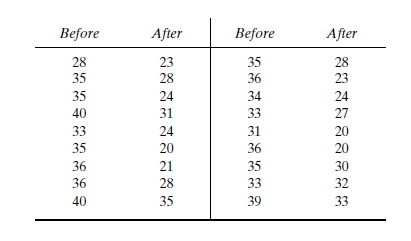
Before an increase in speed enforcement activities:
The speed ranges from 28 to 40 mi/h giving a speed range of 12. For five classes, the range per class is 2.4 mi/h. A frequency distribution table can then be prepared, as shown below in which the speed classes are listed in column 1 and the mid-values are in column 2. The number of observations for each class is listed in column 3 and the cumulative percentages of all observations are listed in column 6.
| 1 | 2 | 3 | 4 | 5 | 6 | 7 |
| Speed class (mi/h) | Class mid-value | Class frequency, | Percentage of class frequency | Cumulative percentage of class frequency | ||
| 28-30 | 29 | 4 | 116 | 13 | 13 | 139.24 |
| 31-33 | 32 | 5 | 160 | 17 | 30 | 42.05 |
| 34-36 | 35 | 12 | 420 | 40 | 70 | 0.12 |
| 37-39 | 38 | 6 | 228 | 20 | 90 | 57.66 |
| 40-42 | 41 | 3 | 123 | 10 | 100 | 111.63 |
| Total | 30 | 1047 | 350.7 |
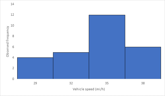
Below Figure shows the frequency histogram for the data shown in above Table. The values in columns 2 and 3 of Table are used to draw the frequency histogram, where the abscissa represents the speeds and the ordinate the observed frequency in each class.

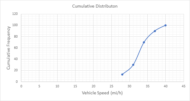
Below Figure shows the cumulative frequency distribution curve for the data given. In this case, the cumulative percentages in column 6 of above Table are plotted against the upper limit of each corresponding speed class. This curve gives the percentage of vehicles that are traveling at or below a given speed.

Determine the arithmetic mean speed:
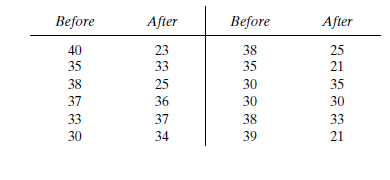
After an increase in speed enforcement activities:
The speed ranges from 20 to 37 mi/h giving a speed range of 17. For six classes, the range per class is 2.83 mi/h. A frequency distribution table can then be prepared, as shown below in which the speed classes are listed in column 1 and the mid-values are in column 2. The number of observations for each class is listed in column 3 and the cumulative percentages of all observations are listed in column 6.
| 1 | 2 | 3 | 4 | 5 | 6 | 7 |
| Speed class (mi/h) | Class mid-value | Class frequency, | Percentage of class frequency | Cumulative percentage of class frequency | ||
| 20-22 | 21 | 6 | 126 | 20 | 20 | 253.5 |
| 23-25 | 24 | 8 | 192 | 27 | 47 | 98 |
| 26-28 | 27 | 4 | 108 | 13 | 60 | 1 |
| 29-31 | 30 | 3 | 90 | 10 | 70 | 18.75 |
| 32-34 | 33 | 5 | 165 | 17 | 87 | 151.25 |
| 35-37 | 36 | 4 | 144 | 13 | 100 | 289 |
| Total | 30 | 825 | 811.5 |
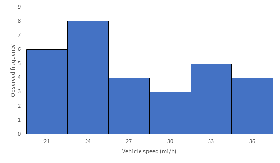
Below Figure shows the frequency histogram for the data shown in above Table. The values in columns 2 and 3 of Table are used to draw the frequency histogram, where the abscissa represents the speeds and the ordinate the observed frequency in each class.

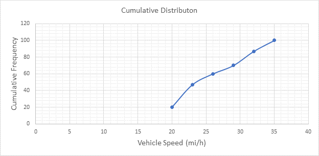
Below Figure shows the cumulative frequency distribution curve for the data given. In this case, the cumulative percentages in column 6 of above Table are plotted against the upper limit of each corresponding speed class. This curve gives the percentage of vehicles that are traveling at or below a given speed.

Determine the arithmetic mean speed:
Conclusion:
The average speeds of each set of data are 34.9 and 27.5 mi/h respectively.
(b)
The histogram frequency distribution, cumulative percentage distribution for each set of data and 85th percentile speed.
Answer to Problem 10P
Explanation of Solution
Given:
Significance level of

Calculation:
Before an increase in speed enforcement activities:
The speed ranges from 28 to 40 mi/h giving a speed range of 12. For five classes, the range per class is 2.4 mi/h. A frequency distribution table can then be prepared, as shown below in which the speed classes are listed in column 1 and the mid-values are in column 2. The number of observations for each class is listed in column 3 and the cumulative percentages of all observations are listed in column 6.
| 1 | 2 | 3 | 4 | 5 | 6 | 7 |
| Speed class (mi/h) | Class mid-value | Class frequency, | Percentage of class frequency | Cumulative percentage of class frequency | ||
| 28-30 | 29 | 4 | 116 | 13 | 13 | 139.24 |
| 31-33 | 32 | 5 | 160 | 17 | 30 | 42.05 |
| 34-36 | 35 | 12 | 420 | 40 | 70 | 0.12 |
| 37-39 | 38 | 6 | 228 | 20 | 90 | 57.66 |
| 40-42 | 41 | 3 | 123 | 10 | 100 | 111.63 |
| Total | 30 | 1047 | 350.7 |
Below Figure shows the frequency histogram for the data shown in above Table. The values in columns 2 and 3 of Table are used to draw the frequency histogram, where the abscissa represents the speeds and the ordinate the observed frequency in each class.

Below Figure shows the cumulative frequency distribution curve for the data given. In this case, the cumulative percentages in column 6 of above Table are plotted against the upper limit of each corresponding speed class. This curve gives the percentage of vehicles that are traveling at or below a given speed.

The 85th-percentile speed is obtained from the cumulative frequency distribution curve as 36 mi/h.
After an increase in speed enforcement activities:
The speed ranges from 20 to 37 mi/h giving a speed range of 17. For six classes, the range per class is 2.83 mi/h. A frequency distribution table can then be prepared, as shown below in which the speed classes are listed in column 1 and the mid-values are in column 2. The number of observations for each class is listed in column 3 and the cumulative percentages of all observations are listed in column 6.
| 1 | 2 | 3 | 4 | 5 | 6 | 7 |
| Speed class (mi/h) | Class mid-value | Class frequency, | Percentage of class frequency | Cumulative percentage of class frequency | ||
| 20-22 | 21 | 6 | 126 | 20 | 20 | 253.5 |
| 23-25 | 24 | 8 | 192 | 27 | 47 | 98 |
| 26-28 | 27 | 4 | 108 | 13 | 60 | 1 |
| 29-31 | 30 | 3 | 90 | 10 | 70 | 18.75 |
| 32-34 | 33 | 5 | 165 | 17 | 87 | 151.25 |
| 35-37 | 36 | 4 | 144 | 13 | 100 | 289 |
| Total | 30 | 825 | 811.5 |
Below Figure shows the frequency histogram for the data shown in above Table. The values in columns 2 and 3 of Table are used to draw the frequency histogram, where the abscissa represents the speeds and the ordinate the observed frequency in each class.

Below Figure shows the cumulative frequency distribution curve for the data given. In this case, the cumulative percentages in column 6 of above Table are plotted against the upper limit of each corresponding speed class. This curve gives the percentage of vehicles that are traveling at or below a given speed.

The 85th-percentile speed is obtained from the cumulative frequency distribution curve as 31.5 mi/h.
Conclusion:
The 85th-percentile speed for each set of data are 36 and 31.5 mi/h respectively.
(c)
The histogram frequency distribution, cumulative percentage distribution for each set of data and 15th percentile speed.
Answer to Problem 10P
Explanation of Solution
Given:
Significance level of


Calculation:
Before an increase in speed enforcement activities:
The speed ranges from 28 to 40 mi/h giving a speed range of 12. For five classes, the range per class is 2.4 mi/h. A frequency distribution table can then be prepared, as shown below in which the speed classes are listed in column 1 and the mid-values are in column 2. The number of observations for each class is listed in column 3 and the cumulative percentages of all observations are listed in column 6.
| 1 | 2 | 3 | 4 | 5 | 6 | 7 |
| Speed class (mi/h) | Class mid-value | Class frequency, | Percentage of class frequency | Cumulative percentage of class frequency | ||
| 28-30 | 29 | 4 | 116 | 13 | 13 | 139.24 |
| 31-33 | 32 | 5 | 160 | 17 | 30 | 42.05 |
| 34-36 | 35 | 12 | 420 | 40 | 70 | 0.12 |
| 37-39 | 38 | 6 | 228 | 20 | 90 | 57.66 |
| 40-42 | 41 | 3 | 123 | 10 | 100 | 111.63 |
| Total | 30 | 1047 | 350.7 |
Below Figure shows the frequency histogram for the data shown in above Table. The values in columns 2 and 3 of Table are used to draw the frequency histogram, where the abscissa represents the speeds and the ordinate the observed frequency in each class.
Below Figure shows the cumulative frequency distribution curve for the data given. In this case, the cumulative percentages in column 6 of above Table are plotted against the upper limit of each corresponding speed class. This curve gives the percentage of vehicles that are traveling at or below a given speed.

The 15th-percentile speed is obtained from the cumulative frequency distribution curve as 28.5 mi/h.
After an increase in speed enforcement activities:
The speed ranges from 20 to 37 mi/h giving a speed range of 17. For six classes, the range per class is 2.83 mi/h. A frequency distribution table can then be prepared, as shown below in which the speed classes are listed in column 1 and the mid-values are in column 2. The number of observations for each class is listed in column 3 and the cumulative percentages of all observations are listed in column 6.
| 1 | 2 | 3 | 4 | 5 | 6 | 7 |
| Speed class (mi/h) | Class mid-value | Class frequency, | Percentage of class frequency | Cumulative percentage of class frequency | ||
| 20-22 | 21 | 6 | 126 | 20 | 20 | 253.5 |
| 23-25 | 24 | 8 | 192 | 27 | 47 | 98 |
| 26-28 | 27 | 4 | 108 | 13 | 60 | 1 |
| 29-31 | 30 | 3 | 90 | 10 | 70 | 18.75 |
| 32-34 | 33 | 5 | 165 | 17 | 87 | 151.25 |
| 35-37 | 36 | 4 | 144 | 13 | 100 | 289 |
| Total | 30 | 825 | 811.5 |
Below Figure shows the frequency histogram for the data shown in above Table. The values in columns 2 and 3 of Table are used to draw the frequency histogram, where the abscissa represents the speeds and the ordinate the observed frequency in each class.
Below Figure shows the cumulative frequency distribution curve for the data given. In this case, the cumulative percentages in column 6 of above Table are plotted against the upper limit of each corresponding speed class. This curve gives the percentage of vehicles that are traveling at or below a given speed.
The 15th-percentile speed is obtained from the cumulative frequency distribution curve as 0 mi/h.
Conclusion:
The 15th-percentile speed for each set of data are 28.5 and 0 mi/h respectively.
(d)
The histogram frequency distribution, cumulative percentage distribution for each set of data and mode.
Answer to Problem 10P
35 mi/h and 24 mi/h
Explanation of Solution
Given:
Significance level of


Calculation:
Before an increase in speed enforcement activities:
The speed ranges from 28 to 40 mi/h giving a speed range of 12. For five classes, the range per class is 2.4 mi/h. A frequency distribution table can then be prepared, as shown below in which the speed classes are listed in column 1 and the mid-values are in column 2. The number of observations for each class is listed in column 3 and the cumulative percentages of all observations are listed in column 6.
| 1 | 2 | 3 | 4 | 5 | 6 | 7 |
| Speed class (mi/h) | Class mid-value | Class frequency, | Percentage of class frequency | Cumulative percentage of class frequency | ||
| 28-30 | 29 | 4 | 116 | 13 | 13 | 139.24 |
| 31-33 | 32 | 5 | 160 | 17 | 30 | 42.05 |
| 34-36 | 35 | 12 | 420 | 40 | 70 | 0.12 |
| 37-39 | 38 | 6 | 228 | 20 | 90 | 57.66 |
| 40-42 | 41 | 3 | 123 | 10 | 100 | 111.63 |
| Total | 30 | 1047 | 350.7 |
Below Figure shows the frequency histogram for the data shown in above Table. The values in columns 2 and 3 of Table are used to draw the frequency histogram, where the abscissa represents the speeds and the ordinate the observed frequency in each class.

Below Figure shows the cumulative frequency distribution curve for the data given. In this case, the cumulative percentages in column 6 of above Table are plotted against the upper limit of each corresponding speed class. This curve gives the percentage of vehicles that are traveling at or below a given speed.

The mode or modal speed is obtained from the frequency histogram as 35 mi/h
After an increase in speed enforcement activities:
The speed ranges from 20 to 37 mi/h giving a speed range of 17. For six classes, the range per class is 2.83 mi/h. A frequency distribution table can then be prepared, as shown below in which the speed classes are listed in column 1 and the mid-values are in column 2. The number of observations for each class is listed in column 3 and the cumulative percentages of all observations are listed in column 6.
| 1 | 2 | 3 | 4 | 5 | 6 | 7 |
| Speed class (mi/h) | Class mid-value | Class frequency, | Percentage of class frequency | Cumulative percentage of class frequency | ||
| 20-22 | 21 | 6 | 126 | 20 | 20 | 253.5 |
| 23-25 | 24 | 8 | 192 | 27 | 47 | 98 |
| 26-28 | 27 | 4 | 108 | 13 | 60 | 1 |
| 29-31 | 30 | 3 | 90 | 10 | 70 | 18.75 |
| 32-34 | 33 | 5 | 165 | 17 | 87 | 151.25 |
| 35-37 | 36 | 4 | 144 | 13 | 100 | 289 |
| Total | 30 | 825 | 811.5 |
Below Figure shows the frequency histogram for the data shown in above Table. The values in columns 2 and 3 of Table are used to draw the frequency histogram, where the abscissa represents the speeds and the ordinate the observed frequency in each class.

Below Figure shows the cumulative frequency distribution curve for the data given. In this case, the cumulative percentages in column 6 of above Table are plotted against the upper limit of each corresponding speed class. This curve gives the percentage of vehicles that are traveling at or below a given speed.

The mode or modal speed is obtained from the frequency histogram as 24 mi/h.
Conclusion:
The mode for each set of data are 35 and 24 mi/h respectively.
(e)
The histogram frequency distribution, cumulative percentage distribution for each set of data and median.
Answer to Problem 10P
32.5 and 23.5 mi/h
Explanation of Solution
Given:
Significance level of


Calculation:
Before an increase in speed enforcement activities:
The speed ranges from 28 to 40 mi/h giving a speed range of 12. For five classes, the range per class is 2.4 mi/h. A frequency distribution table can then be prepared, as shown below in which the speed classes are listed in column 1 and the mid-values are in column 2. The number of observations for each class is listed in column 3 and the cumulative percentages of all observations are listed in column 6.
| 1 | 2 | 3 | 4 | 5 | 6 | 7 |
| Speed class (mi/h) | Class mid-value | Class frequency, | Percentage of class frequency | Cumulative percentage of class frequency | ||
| 28-30 | 29 | 4 | 116 | 13 | 13 | 139.24 |
| 31-33 | 32 | 5 | 160 | 17 | 30 | 42.05 |
| 34-36 | 35 | 12 | 420 | 40 | 70 | 0.12 |
| 37-39 | 38 | 6 | 228 | 20 | 90 | 57.66 |
| 40-42 | 41 | 3 | 123 | 10 | 100 | 111.63 |
| Total | 30 | 1047 | 350.7 |
Below Figure shows the frequency histogram for the data shown in above Table. The values in columns 2 and 3 of Table are used to draw the frequency histogram, where the abscissa represents the speeds and the ordinate the observed frequency in each class.

Below Figure shows the cumulative frequency distribution curve for the data given. In this case, the cumulative percentages in column 6 of above Table are plotted against the upper limit of each corresponding speed class. This curve gives the percentage of vehicles that are traveling at or below a given speed.

The median speed is obtained from the cumulative frequency distribution curve as 32.5 mi/h which is the 50th percentile speed.
After an increase in speed enforcement activities:
The speed ranges from 20 to 37 mi/h giving a speed range of 17. For six classes, the range per class is 2.83 mi/h. A frequency distribution table can then be prepared, as shown below in which the speed classes are listed in column 1 and the mid-values are in column 2. The number of observations for each class is listed in column 3 and the cumulative percentages of all observations are listed in column 6.
| 1 | 2 | 3 | 4 | 5 | 6 | 7 |
| Speed class (mi/h) | Class mid-value | Class frequency, | Percentage of class frequency | Cumulative percentage of class frequency | ||
| 20-22 | 21 | 6 | 126 | 20 | 20 | 253.5 |
| 23-25 | 24 | 8 | 192 | 27 | 47 | 98 |
| 26-28 | 27 | 4 | 108 | 13 | 60 | 1 |
| 29-31 | 30 | 3 | 90 | 10 | 70 | 18.75 |
| 32-34 | 33 | 5 | 165 | 17 | 87 | 151.25 |
| 35-37 | 36 | 4 | 144 | 13 | 100 | 289 |
| Total | 30 | 825 | 811.5 |
Below Figure shows the frequency histogram for the data shown in above Table. The values in columns 2 and 3 of Table are used to draw the frequency histogram, where the abscissa represents the speeds and the ordinate the observed frequency in each class.

Below Figure shows the cumulative frequency distribution curve for the data given. In this case, the cumulative percentages in column 6 of above Table are plotted against the upper limit of each corresponding speed class. This curve gives the percentage of vehicles that are traveling at or below a given speed.

The median speed is obtained from the cumulative frequency distribution curve as 23.5 mi/h which is the 50th percentile speed.
Conclusion:
The median speed for each set of data are 32.5 and 23.5 mi/h respectively.
(f)
The histogram frequency distribution, cumulative percentage distribution for each set of data and pace.
Answer to Problem 10P
32 to 39 mi/h and 27 to 36 mi/h
Explanation of Solution
Given:
Significance level of


Calculation:
Before an increase in speed enforcement activities:
The speed ranges from 28 to 40 mi/h giving a speed range of 12. For five classes, the range per class is 2.4 mi/h. A frequency distribution table can then be prepared, as shown below in which the speed classes are listed in column 1 and the mid-values are in column 2. The number of observations for each class is listed in column 3 and the cumulative percentages of all observations are listed in column 6.
| 1 | 2 | 3 | 4 | 5 | 6 | 7 |
| Speed class (mi/h) | Class mid-value | Class frequency, | Percentage of class frequency | Cumulative percentage of class frequency | ||
| 28-30 | 29 | 4 | 116 | 13 | 13 | 139.24 |
| 31-33 | 32 | 5 | 160 | 17 | 30 | 42.05 |
| 34-36 | 35 | 12 | 420 | 40 | 70 | 0.12 |
| 37-39 | 38 | 6 | 228 | 20 | 90 | 57.66 |
| 40-42 | 41 | 3 | 123 | 10 | 100 | 111.63 |
| Total | 30 | 1047 | 350.7 |
Below Figure shows the frequency histogram for the data shown in above Table. The values in columns 2 and 3 of Table are used to draw the frequency histogram, where the abscissa represents the speeds and the ordinate the observed frequency in each class.

Below Figure shows the cumulative frequency distribution curve for the data given. In this case, the cumulative percentages in column 6 of above Table are plotted against the upper limit of each corresponding speed class. This curve gives the percentage of vehicles that are traveling at or below a given speed.
Below figure shows the frequency distribution curve for the data given. In this case, a curve showing percentage of observations against speed is drawn by plotting values from column 5 of above Table against the corresponding values in column 2. The total area under this curve is one or 100 percent.
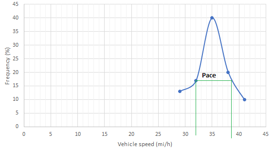
The pace is obtained from the frequency distribution curve above as 32 to 39 mi/h.
After an increase in speed enforcement activities:
The speed ranges from 20 to 37 mi/h giving a speed range of 17. For six classes, the range per class is 2.83 mi/h. A frequency distribution table can then be prepared, as shown below in which the speed classes are listed in column 1 and the mid-values are in column 2. The number of observations for each class is listed in column 3 and the cumulative percentages of all observations are listed in column 6.
| 1 | 2 | 3 | 4 | 5 | 6 | 7 |
| Speed class (mi/h) | Class mid-value | Class frequency, | Percentage of class frequency | Cumulative percentage of class frequency | ||
| 20-22 | 21 | 6 | 126 | 20 | 20 | 253.5 |
| 23-25 | 24 | 8 | 192 | 27 | 47 | 98 |
| 26-28 | 27 | 4 | 108 | 13 | 60 | 1 |
| 29-31 | 30 | 3 | 90 | 10 | 70 | 18.75 |
| 32-34 | 33 | 5 | 165 | 17 | 87 | 151.25 |
| 35-37 | 36 | 4 | 144 | 13 | 100 | 289 |
| Total | 30 | 825 | 811.5 |
Below Figure shows the frequency histogram for the data shown in above Table. The values in columns 2 and 3 of Table are used to draw the frequency histogram, where the abscissa represents the speeds and the ordinate the observed frequency in each class.

Below Figure shows the cumulative frequency distribution curve for the data given. In this case, the cumulative percentages in column 6 of above Table are plotted against the upper limit of each corresponding speed class. This curve gives the percentage of vehicles that are traveling at or below a given speed.

Below figure shows the frequency distribution curve for the data given. In this case, a curve showing percentage of observations against speed is drawn by plotting values from column 5 of above Table against the corresponding values in column 2. The total area under this curve is one or 100 percent.
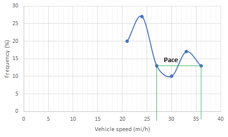
The pace is obtained from the frequency distribution curve drawn above as 27 to 36 mi/h.
Conclusion:
The pace for each set of data are 32 to 39 mi/h and 27 to 36 mi/h respectively.
Want to see more full solutions like this?
Chapter 4 Solutions
Traffic And Highway Engineering


- 5. Two 400 g blocks are connected by a rigid rod. The Blocks can rotate freely at the ends of the rod, so the rod does not apply any moments to the blocks. The blocks are in contact with the wall and floor, and can slide without friction. The system is released from rest when X=24cm and Y=18cm. Ignore the mass of the rod. What are the initial accelerations of Block A and Block B just after being released? Hint: See Assignment 4, Problem 2 for help getting a relationship between the acceleration of Block A and the acceleration of Block B. Y m = 400 g A | L g I 1 I I X B m = 400 garrow_forwardThe momentum of the force F = -100 i -70 j + 50 k around the point O is MO = 410 i- 300 j + 400 k, Determine the coordinates of the point through which the line of actionof F intercepts the yz plane.arrow_forwardAverage sludge production reported by members of the National Association of Clean Water Agencies is 0.7 tons of sludge TS per MG wastewater treated. Assume that the organic matter (VS) in the sludge contains 10% N and that the ratio of VS/TS in sludge is 0.85. A) How many mg/L of N are removed from the wastewater due to assimilation? B) If the raw wastewater contained 50 mg/L total N, what percent was removed via assimilation? C) Why is this a disappointing result in terms of nutrient recovery and reuse goals?arrow_forward
- The two-part curve is from a BOD bottle test conducted over 50 days (i.e., ultimate UBOD). The nitrifying bacteria numbers grew to significance by Day-8.There is a lower cBOD curve and an upper nBOD curve. BOD₁ = UBOD (1− e−k₁t) A) What is the rate constants k for cBOD? B) What is the rate constants k for nBOD? C) Why aren't nitrifiers prevalent in the raw wastewater? Treatment ponds have long hydraulic residence times (HRTs), so nitrifiers are a significant part of the microbiome. D) Sketch a 50-d BOD curve similar to the above, but for a pond effluent sample. The sum of the c and n BODs at 50 days is 30 mg/L. E) Why does your curve have the shape you give it? 100 80 BOD, mg/L 60 60 40 40 20 20 0 0 10 20 30 40 40 Time, d 50 60arrow_forward6-19 Determine the LRFD design strength and the ASD allowable strength of the section shown if snug-tight bolts 3 ft on center are used to connect the A572-Grade 50 angles. The two angles, 5×31/2 × 5/16, are oriented with the long legs back-to-back (2 L5 × 31/2 × 5/16 LLBB) and separated by 3/8 inch. The effective length, (Lc)x = (Lc)y = (Lc)z = 14 ft. (Ans. 65.4 k LRFD; 43.5 k ASD) Figure P6-19 x x 2L5×32×5/16 LLBBarrow_forward6-21 Four 3×3× 1/4 angles are used to form the member shown in the accompanying illustration. The member is 24 ft long, has pinned ends, and consists of A572-Grade 50 steel. Determine the LRFD design strength and the ASD allowable strength of the member. Design single lacing and end tie plates, assuming connections are made to the angles with 3/4-in diameter bolts. (Ans. 159.1 k LRFD; 106.0 k ASD) Figure P6-21 12 in L 12 inarrow_forward
- 1000 th 2' 2' w=200 to /ft Handout Problem #3. A beam has the loading and cross section shown. 1) Draw the shear force and bending moment diagrams for the beam. 5" 2) Determine the maximum bending stress in the beam. Carefully identify its location both along the beam and along the cross section. 3) Determine the maximum transverse shear stress in the beam. Carefully identify its location both along the beam and along the cross section: y=2" up from bottom "INA = 33.33 int VMAX = 1160+b MMAX - 2704 Hb-ft QMAX = 8mm³arrow_forwardUnits: lb-ft Handout Problem #2 The dimensions of the shape as well as the bending moment diagram of a flanged wooden shape are shown. Determine: (a) the maximum tensile bending stress at any location along the beam and (b) the maximum compressive bending stress at any location along the beam. 10 in. 10,580 9,200 4,743 2 in. 8 in. 2 in. 2 in. -8,400 6 in.arrow_forward(USE 0BC 2024) For a 800 m2 4-storey sprinklered Dry-cleaning establishment (not using explosive solvents), facing 1 street(s), what are the minimum required fire-resistance ratings (FRR) or fire-protection ratings (FPR) for the following? Typical floor assembly (in minutes, please. Just write the number of minutes please) Detailed OBC reference = Public corridor wall (in minutes please) Detailed OBC reference = Suite egress door (in minutes, please) = Detailed OBC reference = Exit stair walls (in minutes, please) = Detailed OBC reference = Exit stair door (in minutes, please) = Detailed OBC reference = Elevator shaft enclosure (in minutes, please) = Detailed OBC reference = Vertical mechanical shaft enclosure (in minutes, please) = Detailed OBC reference =arrow_forward
- Question 6 options: The fourth storey of this "Dry-cleaning establishment (not using flammable solvents)" building measures 41 m x 19 m and has a public corridor. Determine the following dimensions, in millimetres (mm) The minimum width of its ramp, if it is sloped at 6°. Please give your answer to the nearest millimetre. The minimum width of its egress doors for Suite D (measuring 6 m × 4 m, ignored the elevator). Please give your answer to the nearest millimetre. The minimum width of its corridor. Please give your answer to the nearest millimetre. The minimum width of its ramp, if it is sloped at 13°. Please give your answer to the nearest millimetre.arrow_forwardFor the exposing building face marked (XX) of this unsprinklered 'Beauty parlours' building, please determine the following. justify THE answer in your hand-written solution.arrow_forwardIf the angle for the sloped glazing below is 45°, is it considered part of the roof or part of the wall? justify the answer with appropriate and detailed OBC references.arrow_forward
 Traffic and Highway EngineeringCivil EngineeringISBN:9781305156241Author:Garber, Nicholas J.Publisher:Cengage Learning
 Residential Construction Academy: House Wiring (M...Civil EngineeringISBN:9781285852225Author:Gregory W FletcherPublisher:Cengage Learning
 Engineering Fundamentals: An Introduction to Engi...Civil EngineeringISBN:9781305084766Author:Saeed MoaveniPublisher:Cengage Learning