
(a)
Estimated regression equation.
(a)
Explanation of Solution
The formula for regression equation is:
Run the ordinary least squares method for the given data in excel. The results drawn are as follows:
Use the summary output to find the estimated regression equation as follows:
(b)
Economic interpretation of each estimated regression coefficients.
(b)
Explanation of Solution
Interpretation of estimated slope (b) coefficient:
For a given level of total no. of rooms, age and attached garage, an additional 100 ft2 will lead to rise in selling price by 3.92×$1000 = $3,920.
For a given level of size, age and attached garage, an additional room will lead to rise in selling price by 3.59×$1000 = $3,590.
For a given level of size, total no. of rooms and attached garage, an additional year of age will lead to fall in selling price by 0.12×$1000 = $120.
For a given level of size, total no. of rooms and age, an additional garage will lead to fall in selling price by 2.83×$1000 = $2,830.
(c)
Statistical significance of the independent variables at 0.05 level.
(c)
Explanation of Solution
Conduct the t-test to know the statistical significance of the independent variables X1, X2, X3 and X4. The test statistic can be calculated using following formula:
The t-statistic follows t-distribution with n-1 degrees of freedom.
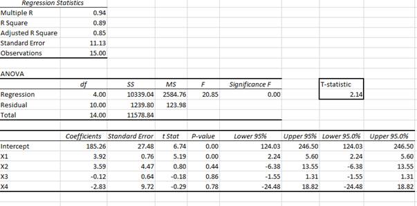
For variable X1, t-test is conducted as follows:
According to the summary output, the t-statistic for X1 variable is equal to 5.19.
At 5% significance level and 15-1= 14 degrees of freedom, the critical value is equal to 2.145.
In figure (1), since the calculated t-statistic lies in the critical region. Therefore, we reject the null hypothesis. This means that the variable X1is statistically significant.
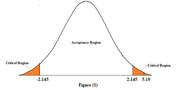
For variable X2, t-test is conducted as follows:
According to the summary output, the t-statistic for X2 variable is equal to 0.80.
At 5% significance level and 15-1= 14 degrees of freedom, the critical value is equal to 2.145.
In figure (2), since the calculated t-statistic lies in the acceptance region. Therefore, we accept the null hypothesis. This means that the variable X2is not statistically significant.
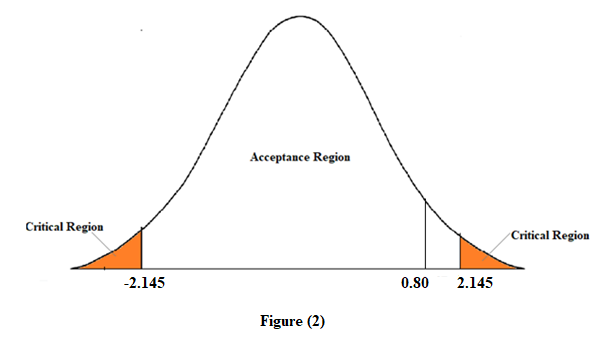
For variable X3, t-test is conducted as follows:
According to the summary output, the t-statistic for X3 variable is equal to -0.18.
At 5% significance level and 15-1= 14 degrees of freedom, the critical value is equal to 2.145.
In figure (3), since the calculated t-statistic lies in the acceptance region. Therefore, we accept the null hypothesis. This means that the variable X3is not statistically significant.
For variable X4, t-test is conducted as follows:
According to the summary output, the t-statistic for X4 variable is equal to -0.29.
At 5% significance level and 15-1= 14 degrees of freedom, the critical value is equal to 2.145.
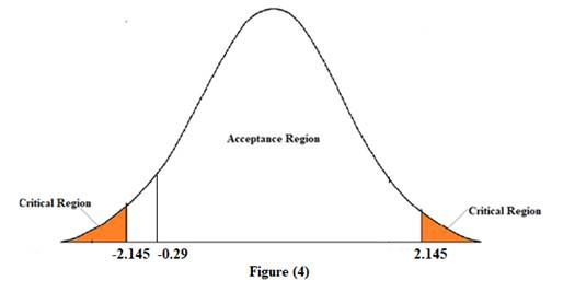
In figure (4), since the calculated t-statistic lies in the acceptance region. Therefore, we accept the null hypothesis. This means that the variable X4is not statistically significant.
(d)
Proportion of total variation in selling price explained by regression model.
(d)
Explanation of Solution
The coefficient of determination measures the proportion of variance predicted by the independent variable in the dependent variable. It is denoted as R2.
According to the summary output, the value of R2 is equal to 0.89. This means that the regression equation predicts 89% of the variance in selling price.
(e)
Overall explanatory power of model by performing F-test at 5 percent level of significance.
(e)
Explanation of Solution
The value of F-statistic is given as 20.85. And the critical value at 0.05 significance level is equal to 0.00.
Since, F-statistic is greater than the critical value. Thus, the overall model is statistically significant.
(f)
95 percent prediction interval for selling price of a 15-year-old house having 1,800 sq. ft., 7 rooms, and an attached garage.
(f)
Explanation of Solution
The confidence interval of a multiple linear regression model can be calculated using following formula:
Here,
y is estimated selling price based on the given values of independent variables
t is critical t value or t-statistic
s.e is multiple standard error of the estimate
The estimated selling price based on the given values of independent variables can be calculated using the estimated regression equation as follows:
According to the regression statistics in the summary output t-statistic and value of multiple standard error of the estimate is equal to 2.14 and 11.13.
Plug the values in the above confidence interval formula as follows:
Thus, an approximate 95% prediction interval for the selling price of a house having an area of a 15-year-old having 1,800 sq. ft., 7 rooms, and an attached garage range from 7291.24 to 7243.60.
Want to see more full solutions like this?
Chapter 4 Solutions
Managerial Economics: Applications, Strategies and Tactics (MindTap Course List)

- In a small open economy with a floating exchange rate, the supply of real money balances is fixed and a rise in government spending ______ Group of answer choices Raises the interest rate so that net exports must fall to maintain equilibrium in the goods market. Cannot change the interest rate so that net exports must fall to maintain equilibrium in the goods market. Cannot change the interest rate so income must rise to maintain equilibrium in the money market Raises the interest rate, so that income must rise to maintain equilibrium in the money market.arrow_forwardSuppose a country with a fixed exchange rate decides to implement a devaluation of its currency and commits to maintaining the new fixed parity. This implies (A) ______________ in the demand for its goods and a monetary (B) _______________. Group of answer choices (A) expansion ; (B) contraction (A) contraction ; (B) expansion (A) expansion ; (B) expansion (A) contraction ; (B) contractionarrow_forwardAssume a small open country under fixed exchanges rate and full capital mobility. Prices are fixed in the short run and equilibrium is given initially at point A. An exogenous increase in public spending shifts the IS curve to IS'. Which of the following statements is true? Group of answer choices A new equilibrium is reached at point B. The TR curve will shift down until it passes through point B. A new equilibrium is reached at point C. Point B can only be reached in the absence of capital mobility.arrow_forward
- A decrease in money demand causes the real interest rate to _____ and output to _____ in the short run, before prices adjust to restore equilibrium. Group of answer choices rise; rise fall; fall fall; rise rise; fallarrow_forwardIf a country's policy makers were to continously use expansionary monetary policy in an attempt to hold unemployment below the natural rate , the long urn result would be? Group of answer choices a decrease in the unemployment rate an increase in the level of output All of these an increase in the rate of inflationarrow_forwardA shift in the Aggregate Supply curve to the right will result in a move to a point that is southwest of where the economy is currently at. Group of answer choices True Falsearrow_forward
- An oil shock can cause stagflation, a period of higher inflation and higher unemployment. When this happens, the economy moves to a point to the northeast of where it currently is. After the economy has moved to the northeast, the Federal Reserve can reduce that inflation without having to worry about causing more unemployment. Group of answer choices True Falsearrow_forwardThe long-run Phillips Curve is vertical which indicates Group of answer choices that in the long-run, there is no tradeoff between inflation and unemployment. that in the long-run, there is no tradeoff between inflation and the price level. None of these that in the long-run, the economy returns to a 4 percent level of inflation.arrow_forwardSuppose the exchange rate between the British pound and the U.S. dollar is £1 = $2.00. The U.S. government implementsU.S. government implements a contractionary fiscal policya contractionary fiscal policy. Illustrate the impact of this change in the market for pounds. 1.) Using the line drawing tool, draw and label a new demand line. 2.) Using the line drawing tool, draw and label a new supply line. Note: Carefully follow the instructions above and only draw the required objects.arrow_forward
- Just Part D please, this is for environmental economicsarrow_forward3. Consider a single firm that manufactures chemicals and generates pollution through its emissions E. Researchers have estimated the MDF and MAC curves for the emissions to be the following: MDF = 4E and MAC = 125 – E Policymakers have decided to implement an emissions tax to control pollution. They are aware that a constant per-unit tax of $100 is an efficient policy. Yet they are also aware that this policy is not politically feasible because of the large tax burden it places on the firm. As a result, policymakers propose a two- part tax: a per unit tax of $75 for the first 15 units of emissions an increase in the per unit tax to $100 for all further units of emissions With an emissions tax, what is the general condition that determines how much pollution the regulated party will emit? What is the efficient level of emissions given the above MDF and MAC curves? What are the firm's total tax payments under the constant $100 per-unit tax? What is the firm's total cost of compliance…arrow_forward2. Answer the following questions as they relate to a fishery: Why is the maximum sustainable yield not necessarily the optimal sustainable yield? Does the same intuition apply to Nathaniel's decision of when to cut his trees? What condition will hold at the equilibrium level of fishing in an open-access fishery? Use a graph to explain your answer, and show the level of fishing effort. Would this same condition hold if there was only one boat in the fishery? If not, what condition will hold, and why is it different? Use the same graph to show the single boat's level of effort. Suppose you are given authority to solve the open-access problem in the fishery. What is the key problem that you must address with your policy?arrow_forward
 Managerial Economics: Applications, Strategies an...EconomicsISBN:9781305506381Author:James R. McGuigan, R. Charles Moyer, Frederick H.deB. HarrisPublisher:Cengage Learning


