
(a)
Estimated regression line.
(a)
Explanation of Solution
The formula for the regression equation is:
Run the ordinary least squares method for the given data in excel. The results drawn are as follows:
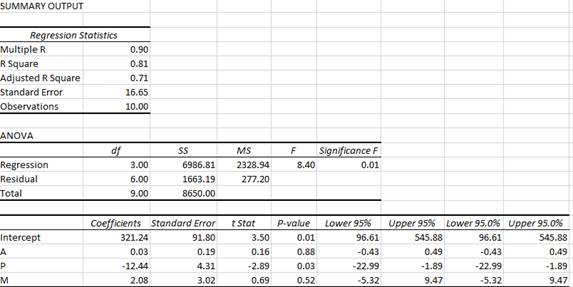
Use the summary output to find the estimated regression equation as follows:
(b)
The economic interpretation of the estimated intercept (a) and slope (b) coefficients.
(b)
Explanation of Solution
Interpretation of estimated intercept (a) coefficient:
When the selling
Interpretation of estimated slope (b) coefficient:
For a given level of selling price and disposable income, an additional $1,000 promotional expenditures lead to a rise in sales by 0.03×1000 = 30 gallons on average.
For a given level of promotional expenditure and selling price, an additional $1,000 disposable income leads to a rise in sales by 2.08×1000 = 2,080 gallons on an average.
For a given level of promotional expenditure and disposable income, an additional $1/gallon lead to falling in sales by 12.44×1000 = 12,440 gallons on an average.
(c)
The hypothesis that there is no relationship between the variables at 0.05 significance level.
(c)
Explanation of Solution
Conduct the t-test to know the statistical significance of the independent variables A, Pand M. The test statistic can be calculated using the following formula:
The t-statistic follows t-distribution with n-1 degrees of freedom.
For variable A, t-test is conducted as follows:
According to the summary output, the t-statistic for A variable is equal to 0.16.
At 5% significance level and 10-1=9 degrees of freedom, the critical value is equal to 2.262.
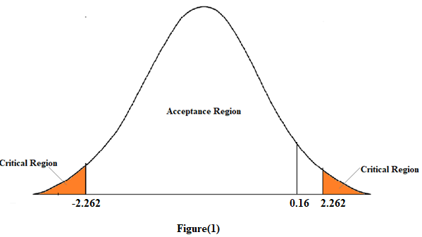
In figure (1), since the calculated t-statistic lies in the acceptance region. Therefore, we accept the null hypothesis. This means that the variable A is not statistically significant.
For variable P, t-test is conducted as follows:
According to the summary output, the t-statistic for P variable is equal to -2.89. At 5% significance level and 10-1=9 degrees of freedom, the critical value is equal to 2.262.
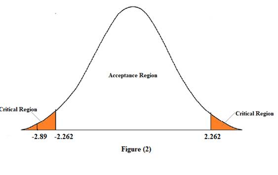
In figure (2), since the calculated t-statistic lies in the critical region. Therefore, we reject the null hypothesis. This means that the variable Pis statistically significant.
For variable M, t-test is conducted as follows:
According to the summary output, the t-statistic for M variable is equal to 0.69.
At 5% significance level and 10-1=9 degrees of freedom, the critical value is equal to 2.262.
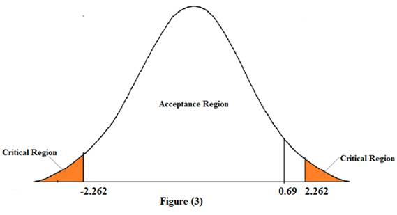
In figure (3), since the calculated t-statistic lies in the acceptance region. Therefore, we accept the null hypothesis. This means that the M variable is not statistically significant.
(d)
Coefficient of determination.
(d)
Explanation of Solution
The coefficient of determination measures the proportion of variance predicted by the independent variable in the dependent variable. It is denoted as R2.
According to the summary output, the value of R2 is equal to 0.81. This means that the regression equation predicts 81% of the variance in sales.
(e)
(e)
Explanation of Solution
The value of F-statistic is given as 8.40. And the critical value at 0.05 significance level is equal to 0.01.
Since F-statistic is greater than the critical value, thus, the overall model is statistically significant.
(f)
Best estimate of the product sales when the selling price is $14.50. And an approximate 95 percent prediction interval.
(f)
Explanation of Solution
According to the regression statistics of the summary output, for a given level of promotional expenditure and disposable income, $14.50/gallon lead to fall in sales by 12.44×14.50×1000 = 180,380 gallons on an average.
According to the regression statistics in the summary output, a 95% confidence interval for the P variable ranges from -22.99 to -1.89.
(g)
(g)
Explanation of Solution
Formula to calculate elasticity in linear regression model is as follows:
At given value of P variable equal to 14.50, the estimated value of Y variable is equal to 180,380.
Thus, price
Thus, the price elasticity of demand at a selling price of $14.50 is equal to -0.001.
Want to see more full solutions like this?
Chapter 4 Solutions
Managerial Economics: Applications, Strategies and Tactics (MindTap Course List)

- a-c pleasearrow_forwardd-farrow_forwardPART II: Multipart Problems wood or solem of triflussd aidi 1. Assume that a society has a polluting industry comprising two firms, where the industry-level marginal abatement cost curve is given by: MAC = 24 - ()E and the marginal damage function is given by: MDF = 2E. What is the efficient level of emissions? b. What constant per-unit emissions tax could achieve the efficient emissions level? points) c. What is the net benefit to society of moving from the unregulated emissions level to the efficient level? In response to industry complaints about the costs of the tax, a cap-and-trade program is proposed. The marginal abatement cost curves for the two firms are given by: MAC=24-E and MAC2 = 24-2E2. d. How could a cap-and-trade program that achieves the same level of emissions as the tax be designed to reduce the costs of regulation to the two firms?arrow_forward
- Only #4 please, Use a graph please if needed to help provearrow_forwarda-carrow_forwardFor these questions, you must state "true," "false," or "uncertain" and argue your case (roughly 3 to 5 sentences). When appropriate, the use of graphs will make for stronger answers. Credit will depend entirely on the quality of your explanation. 1. If the industry facing regulation for its pollutant emissions has a lot of political capital, direct regulatory intervention will be more viable than an emissions tax to address this market failure. 2. A stated-preference method will provide a measure of the value of Komodo dragons that is more accurate than the value estimated through application of the travel cost model to visitation data for Komodo National Park in Indonesia. 3. A correlation between community demographics and the present location of polluting facilities is sufficient to claim a violation of distributive justice. olsvrc Q 4. When the damages from pollution are uncertain, a price-based mechanism is best equipped to manage the costs of the regulator's imperfect…arrow_forward
- For environmental economics, question number 2 only please-- thank you!arrow_forwardFor these questions, you must state "true," "false," or "uncertain" and argue your case (roughly 3 to 5 sentences). When appropriate, the use of graphs will make for stronger answers. Credit will depend entirely on the quality of your explanation. 1. If the industry facing regulation for its pollutant emissions has a lot of political capital, direct regulatory intervention will be more viable than an emissions tax to address this market failure. cullog iba linevoz ve bubivorearrow_forwardExercise 3 The production function of a firm is described by the following equation Q=10,000-3L2 where L stands for the units of labour. a) Draw a graph for this equation. Use the quantity produced in the y-axis, and the units of labour in the x-axis. b) What is the maximum production level? c) How many units of labour are needed at that point? d) Provide one reference with you answer.arrow_forward
- Exercise 1 Consider the market supply curve which passes through the intercept and from which the market equilibrium data is known, this is, the price and quantity of equilibrium PE=50 and QE=2000. Considering those two points, find the equation of the supply. Draw a graph of this line. Provide one reference with your answer. Exercise 2 Considering the previous supply line, determine if the following demand function corresponds to the market demand equilibrium stated above. QD=3000-2p.arrow_forwardConsider the market supply curve which passes through the intercept and from which the marketequilibrium data is known, this is, the price and quantity of equilibrium PE=50 and QE=2000.a. Considering those two points, find the equation of the supply. b. Draw a graph of this line.arrow_forwardGovernment Purchases and Tax Revenues A B GDP T₂ Refer to the diagram. Discretionary fiscal policy designed to slow the economy is illustrated by Multiple Choice the shift of curve T₁ to T2. a movement from d to balong curve T₁.arrow_forward
 Managerial Economics: Applications, Strategies an...EconomicsISBN:9781305506381Author:James R. McGuigan, R. Charles Moyer, Frederick H.deB. HarrisPublisher:Cengage Learning


