
(a)
Units of clothing the consumer is consuming.
Explanation of Solution
The consumer prefers food (F) and clothing (C). The per-unit
Budget constraint depicts different bundles of goods and services that the consumers can purchase at a given level of market prices and their income.
Mathematically, it is expressed as follows:
Here,
'F' represents units of food
'PF'represents price of food ($1)
'C' represents units of clothing
'Pc'represents price of clothing ($2)
'I' represent consumer's income ($22)
Thus, the budget constraint of the consumer is given as follows:
It is given that consumer is consuming 8 units of F. Plug the given value of F equal to 8 in (1) to get the value of C.
Thus, the consumer is consuming 7 units of Clothing.
(b)
To graph the budget line and plot the current consumption of both goods.
Explanation of Solution
Figure (1) below depicts the graph of the consumer's budget constraint 'BC'. Here, X-axis measures the quantity of good 'F' and the Y-axis measures the quantity of good 'C.'
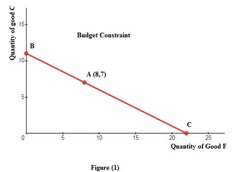
Point A on the budget line BC depicts the current consumption basket of the consumer.
(c)
To graph indifference curves corresponding to utility =36 and utility =72.
Explanation of Solution
The utility function of the consumer is given as follows:
The figure (2) below depicts the graph of indifference curves corresponding to U=36 andU =72. Here, X-axis measures the quantity of good F and the Y-axis measures the quantity of good C.
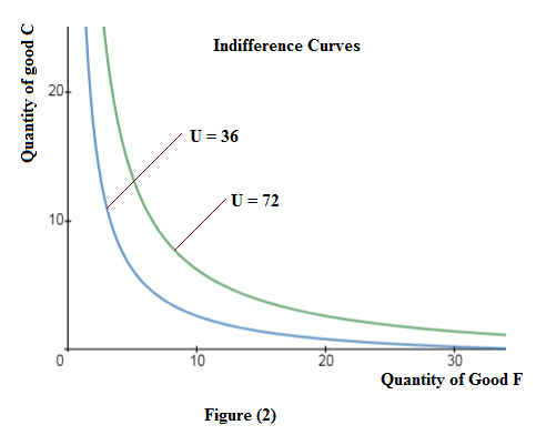
The figure (2) shows that the indifference curves are in toward the origin.
(d)
To graphically show the Utility maximizing choice of the goods.
Explanation of Solution
At the optimal level of consumption, the slope of the indifference curve is equal to the slope of the budget constraint. Graphically, the point at which the budget line is tangent to the indifference curve gives the optimal level of consumption.
The figure (3) below plots the budget constraint along with the indifference curves of the consumer.
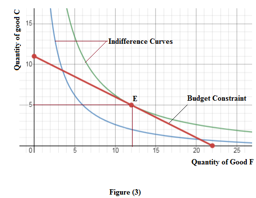
At point E, budget constraint is tangent to indifference curve. Thus, utility maximizing choice of F and C is equal to 12 units and 5 units respectively.
(e)
To find the Utility maximizing choice of the goods using algebra.
Explanation of Solution
The rate at which consumer is willing to sacrifice some units good F to get an additional unit of good C is known as the marginal rate of substitution (MRS).
It measures the slope of the indifference curve.
The ratio of the price of good F to the price of good C measures slope of the budget constraint.
At the optimum level of consumption, the slope of the indifference curve is equal to the slope of the budget constraint. Mathematically, it is expressed as follows:
Also, marginal utilities of the two goods are given as follows:
Plug the given expressions of the marginal utilities and the values of the prices in (2) as follows:
Put (3) in (1).
Plug value of C equal to 5 in (3).
Thus, utility-maximizing choice of F and C is equal to 12 units and 5 units respectively.
(f)
The marginal rate of substitution of F for C when the utility is maximized.
Explanation of Solution
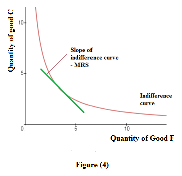
Mathematically, the marginal rate of substitution of F for Cis expressed as the ratio of
Graphically, marginal rate of substitution of F for Cis expressed as slope of indifference curve of the consumer, as shown in figure (4) below:
(g)
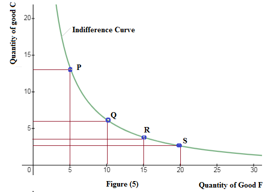
Whether the consumer has a diminishing marginal rate of substitution of F for C.
Explanation of Solution
According to the law of diminishing marginal rate of substitution, the consumer is willing to sacrifice less and fewer units of good C to get an additional unit of good F.
According to figure (5), consumer switches from point Q to point R level of consumption and from point R to point S level of consumption.
Here, the quantity of good F increases by one unit, but the quantity of good C sacrificed decreases.
Thus, it is concluded that the consumer has a diminishing marginal rate of substitution of F for C.
Want to see more full solutions like this?
Chapter 4 Solutions
EBK MICROECONOMICS

- 4. Supply and Demand. The table gives hypothetical data for the quantity of electric scooters demanded and supplied per month. Price per Electric Scooter Quantity Quantity Demanded Supplied $150 500 250 $175 475 350 $200 450 450 $225 425 550 $250 400 650 $275 375 750 a. Graph the demand and supply curves. Note if you prefer to hand draw separately, you may and insert the picture separately. Price per Scooter 300 275 250 225 200 175 150 250 400 375425475 350 450 550 650 750 500 850 Quantity b. Find the equilibrium price and quantity using the graph above. c. Illustrate on your graph how an increase in the wage rate paid to scooter assemblers would affect the market for electric scooters. Label any new lines in the same graph above to distinguish changes. d. What would happen if there was an increase in the wage rate paid to scooter assemblers at the same time that tastes for electric scooters increased? 1ངarrow_forward3. Production Costs Clean 'n' Shine is a competitor to Spotless Car Wash. Like Spotless, it must pay $150 per day for each automated line it uses. But Clean 'n' Shine has been able to tap into a lower-cost pool of labor, paying its workers only $100 per day. Clean 'n' Shine's production technology is given in the following table. To determine its short-run cost structure, fill in the blanks in the table. Fill in the columns below. Outpu Capita Labor TFC TVC TC MC AFC AVC ATC 1 0 30 1 1 70 1 2 120 1 3 160 1 4 190 1 5 210 1 6 a. Over what range of output does Clean 'n' Shine experience increasing marginal returns to labor? Over what range does it experience diminishing marginal returns to labor? (*answer both questions) b. As output increases, do average fixed costs behave as described in the text? Explain. C. As output increases, do marginal cost, average variable cost, and average total cost behave as described in the text? Explain. d. Looking at the numbers in the table, but without…arrow_forward2. Elasticity and the Minimum Wage - The following graph depicts two labor markets for cashiers. We assume the same supply curve (cashiers respond similarly to wage offers in each city) but different demand functions (employer demand is more elastic – more responsive to wages - in one city than the other, perhaps because one has higher quality retail stores than the other). The y-axis shows hourly wages in dollars; the x-axis shows the number of employees in hundreds. Wage 12 11 29 10 9 00 8 7 Supply 5 4 3 2 1 D2 12 D1 0 0 1 2 3 4 5 6 7 8 9 10 11 12 Employment 11 With minimum wage of 8 dollars: A. What is the equilibrium level of employment before the minimum wage is imposed? B. A) According to the graph and given a minimum wage of 8 dollars, how many workers would employers want to hire if the demand for workers in City #1 looked like D1? B) How does that number compare to the market equilibrium employment? C. A) In City #1 (with demand curve D1), would there be an excess supply of…arrow_forward
- The demand function for organic apples is given by Qd = 20 – 2P while the supply function is given by Qs = 4P – 10.a. Solve for the equilibrium P* and Q*.b. Carefully graph the D & S curves. Include all intercepts and P* and Q* (**enlarge your graph so you can better show the questions below use graphing paper**)i. Suppose that the government legislates a $1/gallon to be collected from the buyer. Identify the new equation for the demand curve. Plot the new demand curve (on the same graph as b).ii. Solve for the new equilibrium PT* and QT* and indicate on your graph. On the same graph, indicate the P that consumers pay (PC) and the P that producers get to keep (PS).c. On another graph with the original D and S curves, impose the same tax ($1/gallon) to sellers. Identify the new equation for the supply curve. Plot the new supply curve. i. Solve for the new equilibrium PT* and QT* and indicate on your graph. On thesame graph, indicate the P that consumers pay (PC) and the P that…arrow_forwardDon't use ai to answer I will report you answerarrow_forwardExplain and evaluate the impact of legislation on the U.S. criminal justice system, specifically on the prison population and its impact on poverty and the U.S. economy. Include significant elements and limitations such as the War on Drugs and the First Step Act.arrow_forward
- Given the following petroleum tax details, calculate the marginal tax rate and explain its significance: Total Revenue: $500 million Cost of Operations: $200 million Tax Rate: 40% Additional Royalty: 5% Profit-Based Tax: 10%arrow_forwardUse a game tree to illustrate why an aircraft manufacturer may price below the current marginal cost in the short run if it has a steep learning curve. (Hint: Show that learning by doing lowers its cost in the second period.) Part 2 Assume for simplicity the game tree is illustrated in the figure to the right. Pricing below marginal cost reduces profits but gives the incumbent a cost advantage over potential rivals. What is the subgame perfect Nash equilibrium?arrow_forwardAnswerarrow_forward
- M” method Given the following model, solve by the method of “M”. (see image)arrow_forwardAs indicated in the attached image, U.S. earnings for high- and low-skill workers as measured by educational attainment began diverging in the 1980s. The remaining questions in this problem set use the model for the labor market developed in class to walk through potential explanations for this trend. 1. Assume that there are just two types of workers, low- and high-skill. As a result, there are two labor markets: supply and demand for low-skill workers and supply and demand for high-skill workers. Using two carefully drawn labor-market figures, show that an increase in the demand for high skill workers can explain an increase in the relative wage of high-skill workers. 2. Using the same assumptions as in the previous question, use two carefully drawn labor-market figures to show that an increase in the supply of low-skill workers can explain an increase in the relative wage of high-skill workers.arrow_forwardPublished in 1980, the book Free to Choose discusses how economists Milton Friedman and Rose Friedman proposed a one-sided view of the benefits of a voucher system. However, there are other economists who disagree about the potential effects of a voucher system.arrow_forward
 Exploring EconomicsEconomicsISBN:9781544336329Author:Robert L. SextonPublisher:SAGE Publications, Inc
 Economics (MindTap Course List)EconomicsISBN:9781337617383Author:Roger A. ArnoldPublisher:Cengage Learning

 Microeconomics: Private and Public Choice (MindTa...EconomicsISBN:9781305506893Author:James D. Gwartney, Richard L. Stroup, Russell S. Sobel, David A. MacphersonPublisher:Cengage Learning
 Economics: Private and Public Choice (MindTap Cou...EconomicsISBN:9781305506725Author:James D. Gwartney, Richard L. Stroup, Russell S. Sobel, David A. MacphersonPublisher:Cengage Learning