Concept explainers
Videos
As shown in Figure 4.40, force vector
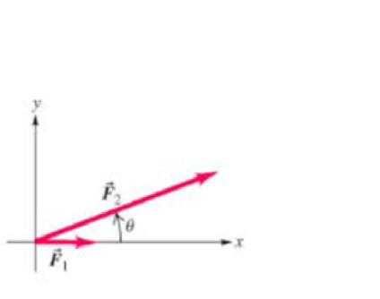
Figure 4.40
Problem 43.
| θ | Fx(N) | Fy(N) |
| 20* | 11.4 | 3.1 |
| 35* | 10.4 | 5.2 |
| 60* | 7.5 | 7.8 |
| 75* | 5.3 | 8.7 |
(a) Write an expression for F in terms of θ F1 and F2. (b) Make a linearized graph of the x component data with the value F, values on the y axis and the appropriate trig function of 0 on the x axis. (c) Draw a best-fit line through your plotted points and use this line to determine the magnitude F1 and F2. (d) Repeat this process for the F1 data and compare your result with what you obtained in part(c).
Want to see the full answer?
Check out a sample textbook solution
Chapter 4 Solutions
College Physics (10th Edition)
Additional Science Textbook Solutions
Brock Biology of Microorganisms (15th Edition)
Physics for Scientists and Engineers: A Strategic Approach, Vol. 1 (Chs 1-21) (4th Edition)
Chemistry: An Introduction to General, Organic, and Biological Chemistry (13th Edition)
Concepts of Genetics (12th Edition)
Applications and Investigations in Earth Science (9th Edition)
Campbell Essential Biology with Physiology (5th Edition)


- An EL NIÑO usually results in Question 8Select one: a. less rainfall for Australia. b. warmer water in the western Pacific. c. all of the above. d. none of the above. e. more rainfall for South America.arrow_forwardEarth’s mantle is Question 12Select one: a. Solid b. Liquid c. Metallic d. very dense gasarrow_forwardSilicates Question 18Select one: a. All of these b. Are minerals c. Consist of tetrahedra d. Contain silicon and oxygenarrow_forward
- Which of the following is not one of the major types of metamorphism? Question 20Select one: a. Fold b. Contact c. Regional d. Sheararrow_forwardA bungee jumper plans to bungee jump from a bridge 64.0 m above the ground. He plans to use a uniform elastic cord, tied to a harness around his body, to stop his fall at a point 6.00 m above the water. Model his body as a particle and the cord as having negligible mass and obeying Hooke's law. In a preliminary test he finds that when hanging at rest from a 5.00 m length of the cord, his body weight stretches it by 1.55 m. He will drop from rest at the point where the top end of a longer section of the cord is attached to the bridge. (a) What length of cord should he use? m (b) What maximum acceleration will he experience? m/s²arrow_forwardOne end of a light spring with spring constant k is attached to the ceiling. A second light spring is attached to the lower end, with spring constant k. An object of mass m is attached to the lower end of the second spring. (a) By how much does the pair of springs stretch? (Use the following as necessary: k₁, k₂, m, and g, the gravitational acceleration.) Xtotal (b) What is the effective spring constant of the spring system? (Use the following as necessary: k₁, k₂, m, and g, the gravitational acceleration.) Keff (c) What If? Two identical light springs with spring constant k3 are now individually hung vertically from the ceiling and attached at each end of a symmetric object, such as a rectangular block with uniform mass density. In this case, with the springs next to each other, we describe them as being in parallel. Find the effective spring constant of the pair of springs as a system in this situation in terms of k3. (Use the following as necessary: k3, M, the mass of the symmetric…arrow_forward
- A object of mass 3.00 kg is subject to a force FX that varies with position as in the figure below. Fx (N) 4 3 2 1 x(m) 2 4 6 8 10 12 14 16 18 20 i (a) Find the work done by the force on the object as it moves from x = 0 to x = 5.00 m. J (b) Find the work done by the force on the object as it moves from x = 5.00 m to x = 11.0 m. ] (c) Find the work done by the force on the object as it moves from x = 11.0 m to x = 18.0 m. J (d) If the object has a speed of 0.400 m/s at x = 0, find its speed at x = 5.00 m and its speed at x speed at x = 5.00 m speed at x = 18.0 m m/s m/s = 18.0 m.arrow_forwardA crate with a mass of 74.0 kg is pulled up an inclined surface by an attached cable, which is driven by a motor. The crate moves a distance of 70.0 m along the surface at a constant speed of 3.3 m/s. The surface is inclined at an angle of 30.0° with the horizontal. Assume friction is negligible. (a) How much work (in kJ) is required to pull the crate up the incline? kJ (b) What power (expressed in hp) must a motor have to perform this task? hparrow_forwardA deli uses an elevator to move items from one level to another. The elevator has a mass of 550 kg and moves upward with constant acceleration for 2.00 s until it reaches its cruising speed of 1.75 m/s. (Note: 1 hp (a) What is the average power (in hp) of the elevator motor during this time interval? Pave = hp (b) What is the motor power (in hp) when the elevator moves at its cruising speed? Pcruising hp = 746 W.)arrow_forward
- A 1.40-kg object slides to the right on a surface having a coefficient of kinetic friction 0.250 (Figure a). The object has a speed of v₁ = 3.50 m/s when it makes contact with a light spring (Figure b) that has a force constant of 50.0 N/m. The object comes to rest after the spring has been compressed a distance d (Figure c). The object is then forced toward the left by the spring (Figure d) and continues to move in that direction beyond the spring's unstretched position. Finally, the object comes to rest a distance D to the left of the unstretched spring (Figure e). d m v=0 -D- www (a) Find the distance of compression d (in m). m (b) Find the speed v (in m/s) at the unstretched position when the object is moving to the left (Figure d). m/s (c) Find the distance D (in m) where the object comes to rest. m (d) What If? If the object becomes attached securely to the end of the spring when it makes contact, what is the new value of the distance D (in m) at which the object will come to…arrow_forwardAs shown in the figure, a 0.580 kg object is pushed against a horizontal spring of negligible mass until the spring is compressed a distance x. The force constant of the spring is 450 N/m. When it is released, the object travels along a frictionless, horizontal surface to point A, the bottom of a vertical circular track of radius R = 1.00 m, and continues to move up the track. The speed of the object at the bottom of the track is VA = 13.0 m/s, and the object experiences an average frictional force of 7.00 N while sliding up the track. R (a) What is x? m A (b) If the object were to reach the top of the track, what would be its speed (in m/s) at that point? m/s (c) Does the object actually reach the top of the track, or does it fall off before reaching the top? O reaches the top of the track O falls off before reaching the top ○ not enough information to tellarrow_forwardA block of mass 1.4 kg is attached to a horizontal spring that has a force constant 900 N/m as shown in the figure below. The spring is compressed 2.0 cm and is then released from rest. wwww wwwwww a F x = 0 0 b i (a) A constant friction force of 4.4 N retards the block's motion from the moment it is released. Using an energy approach, find the position x of the block at which its speed is a maximum. ст (b) Explore the effect of an increased friction force of 13.0 N. At what position of the block does its maximum speed occur in this situation? cmarrow_forward
 Principles of Physics: A Calculus-Based TextPhysicsISBN:9781133104261Author:Raymond A. Serway, John W. JewettPublisher:Cengage Learning
 Classical Dynamics of Particles and SystemsPhysicsISBN:9780534408961Author:Stephen T. Thornton, Jerry B. MarionPublisher:Cengage Learning
 University Physics Volume 1PhysicsISBN:9781938168277Author:William Moebs, Samuel J. Ling, Jeff SannyPublisher:OpenStax - Rice University
 College PhysicsPhysicsISBN:9781305952300Author:Raymond A. Serway, Chris VuillePublisher:Cengage Learning
 Physics for Scientists and Engineers: Foundations...PhysicsISBN:9781133939146Author:Katz, Debora M.Publisher:Cengage Learning
 College PhysicsPhysicsISBN:9781285737027Author:Raymond A. Serway, Chris VuillePublisher:Cengage Learning