Chapter 4, Problem 4.1TI

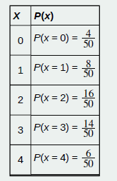
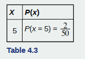
A hospital researcher Is Interested In the number of times the average post-op patient will ring the nurse during a 12-hour shift. For a random sample of 50 patients, the following information was obtained. Let X = the number of times a patient rings the nurse during a 12-hour shift. For this exercise. x = 0, 1, 2, 3. 4, 5. P(x) = the probability that X takes on value x. Why Is this a discrete probability distribution function (two reasons)?

To determine

Why is this a discrete probability distribution (two reasons).

Answer to Problem 4.1TI

The two reasons this is a discrete probability distribution are:

1. Each probability is between zero and one.
2. The sum of probabilities is one.

Explanation of Solution

Given:

A hospital researcher is interested in the number of times the average post-op patient will ring the nurse during a 12-hour shift. For a random sample of 50 patients, the following information was obtained. Let X = the number of times a patient rings the nurse during a 12-hour shift.

$X$	$P(X)$
$0$	$P(x=0)=\frac{4}{50}=0.08$
$1$	$P(x=1)=\frac{8}{50}=0.16$
$2$	$P(x=2)=\frac{16}{50}=0.32$
$3$	$P(x=3)=\frac{14}{50}=0.28$
$4$	$P(x=4)=\frac{6}{50}=0.12$
$5$	$P(x=5)=\frac{2}{50}=0.04$
	${\displaystyle \sum P(x)=1}$

Concept Used:

In statistic, discrete probability distribution is the one which describes the probability of happening of each value of discrete random variable. A discrete random variable is a random variable that has countable values such as the outcomes of dice related to rolling a dice once. A discrete probability distribution has two characteristics and these are:

1. Each probability is between zero and one, inclusive.
2. The sum of probabilities is one.

In the given problem, we are given the probability distribution of random variable the number of times a patient rings the nurse during a 12-hour shift. Now, let’s check these two characteristics.

We clearly see all the probabilities of the given random variable is between zero and one.

The sum of probabilities is:

$\frac{4}{50}+\frac{8}{50}+\frac{16}{50}+\frac{14}{50}+\frac{6}{50}+\frac{2}{50}=\frac{50}{50}=1$

Therefore, the two reasons to consider the given probability distribution are:

1. Each probability of the given random experiment is between zero and one.
2. The sum of probabilities of the given random experiment is one.