Concept explainers
Videos
a.
Construct box plot of the variable price.
Identify whether there are outliers or not.
Find the
Find the first
Find the third quartile value.
a.
Answer to Problem 37CE
Output of box plot for the variable price using MINITAB software is,
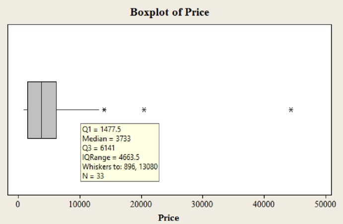
Yes, there are 3 outliers in the dataset.
The median price is 3,733.
The first quartile value is 1,478.
The third quartile value is 6,141.
Explanation of Solution
Calculation:
Step by step procedure to obtain boxplot using MINITAB software is given as,
- Choose Graph > Boxplot.
- In Graph variables enter the columns Price.
- Click OK.
Outliers:
In the boxplot, the outlier is represented using asterisk. In the boxplot of data set there are 3 asterisks representing outliers. Hence, there are three outliers in the dataset.
Median:
The median is the middle value of the data set. In the boxplot, the line in middle of the box represents median of the dataset. The line corresponds to value 3,733.
Hence, the median value is 3,733.
First quartile:
The border line towards the left side of the box represents the value of first quartile. In this box plot, the line of the box on left side corresponds to the value approximately 1,478.
Hence, the third quartile value is 6,141.
Third quartile:
The border line towards the right side of the box represents the value of third quartile. In this box plot, the line of the box on right side corresponds to the value approximately 6,141.
Hence, the first quartile value is 1,478.
b.
Construct box plot of the variable size.
Identify whether there are outliers or not.
Find the median price.
Find the first quartile value.
Find the third quartile value.
b.
Answer to Problem 37CE
Output of box plot for the variable size using MINITAB software is,
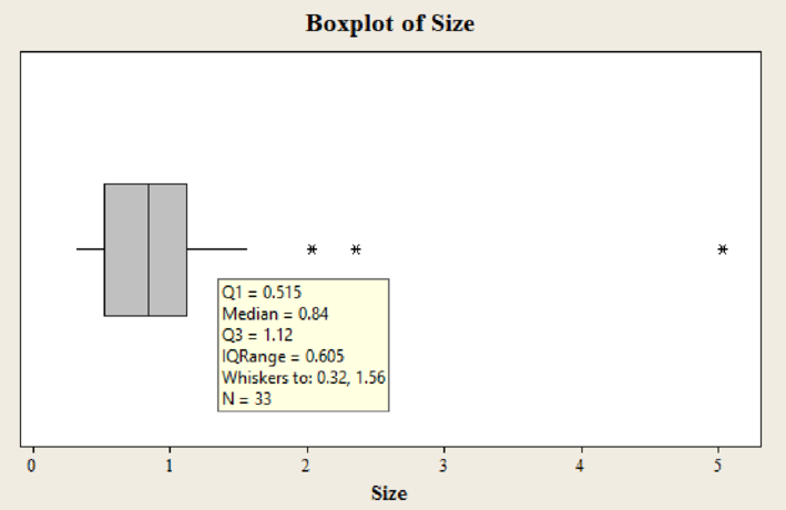
Yes, there are 3 outliers in the dataset.
The median price is 0.84.
The first quartile value is 0.515.
The third quartile value is 1.12.
Explanation of Solution
Calculation:
Step by step procedure to obtain boxplot using MINITAB software is given as,
- Choose Graph > Boxplot.
- In Graph variables enter the columns Size.
- Click OK.
Outliers:
In the boxplot, the outlier is represented using asterisk. In the boxplot of data set there are 3 asterisks representing outliers. Hence, there are three outliers in the dataset.
Median:
The median is the middle value of the data set. In the boxplot, the line in middle of the box represents median of the dataset. The line corresponds to value 0.84.
Hence, the median value is 0.84.
First quartile:
The border line towards the left side of the box represents the value of first quartile. In this box plot, the line of the box on left side corresponds to the value approximately 0.515.
Hence, the third quartile value is 0.515.
Third quartile:
The border line towards the right side of the box represents the value of third quartile. In this box plot, the line of the box on right side corresponds to the value approximately 1.12.
Hence, the first quartile value is 1.12.
c.
Construct
Identify whether there is association between the two variables or not.
Identify whether association is direct or indirect.
Identify whether any point seems to be different from the others.
c.
Answer to Problem 37CE
Output of scatter diagram for variables price and size using MINITAB software is,
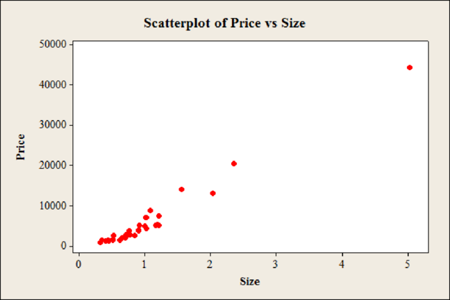
Yes, there is association between the variables price and size.
The association is direct.
Yes, the first observation of both the price and size is large when compared to other observations.
Explanation of Solution
Calculation:
Step by step procedure to obtain scatter diagram using MINITAB software is given as,
- Choose Graph > Scatterplot > select Simple.
- In Y variable enter the column Price.
- In X variable enter the column Size.
- Click OK.
In the scatter diagram it can be observed that, the Price has increased as the Size increases indicating that the association between the variables.
Hence, there is association between the variables price and size
The relation is said to be direct if value of one variable increases due to effect of another variable. From the scatter diagram, the value of Price has increased as the Size increases indicating a direct or positive association.
Hence, the association is direct.
From the scatter diagram, it can be observed that one of the observations corresponding to the value of 5.03 carats for size and $44,312 for price is far from all the other observations. Hence, one point seems to be different from the others.
d.
Construct a
Find the most common cut grade.
Find the most common shape.
Find the most common combination of cut grade and shape.
d.
Answer to Problem 37CE
The contingency table for the variables shape and cut grade is,
| Shape | Cut Grade | |||||
| Average | Good | Ideal | Premium | Ultra Ideal | Total | |
| Emerald | 0 | 0 | 1 | 0 | 0 | 1 |
| Marquise | 0 | 2 | 0 | 1 | 0 | 3 |
| Oval | 0 | 0 | 0 | 1 | 0 | 1 |
| Princess | 1 | 0 | 2 | 2 | 0 | 5 |
| Round | 1 | 3 | 3 | 13 | 3 | 23 |
| Total | 2 | 5 | 6 | 17 | 3 | 33 |
The most common cut grade is premium.
The most common shape is round.
The most common combination of cut grade and shape is premium and round.
Explanation of Solution
Calculation:
Contingency table:
A table that is used for classifying observations based on the two identifiable characteristics is termed as contingency table. It is used for summarizing two variables.
The variable cut grade is classified into 5 different categories ‘average, good, ideal, premium, ultra ideal’. The variable shape is classified into 5 different categories ‘emerald, marquise, oval, princess, and round’.
Count the number of cut grades are average with shape of emerald. From the data, there is no combination of average cut grades with shape of emerald. Hence, the frequency is 0.
Similarly, count the frequency for each of the possible combination of cut grade and shape. Then calculate the totals for each column and row. The contingency table is obtained as below,
| Shape | Cut Grade | |||||
| Average | Good | Ideal | Premium | Ultra Ideal | Total | |
| Emerald | 0 | 0 | 1 | 0 | 0 | 1 |
| Marquise | 0 | 2 | 0 | 1 | 0 | 3 |
| Oval | 0 | 0 | 0 | 1 | 0 | 1 |
| Princess | 1 | 0 | 2 | 2 | 0 | 5 |
| Round | 1 | 3 | 3 | 13 | 3 | 23 |
| Total | 2 | 5 | 6 | 17 | 3 | 33 |
The cut grade ‘Premium’ has a total of 17, which is large when compared to other cut grades. This shows that, the most common cut grade of diamonds is ‘Premium.
Hence, the most common cut grade is premium.
The shape ‘Round’ has a total of 23, which is large when compared to other shapes. This shows that, the most common shape of diamonds is ‘Round’.
Hence, the most common shape is round.
The combination of cut grade ‘Premium’ and shape ‘Round’ has a total of 13, which is large when compared to other combinations. This shows that, the most common combination of diamonds is cut grade ‘Premium’ and shape ‘Round’.
Hence, the most common combination of cut grade and shape is premium and round.
Want to see more full solutions like this?
Chapter 4 Solutions
Loose Leaf for Statistical Techniques in Business and Economics


- A company found that the daily sales revenue of its flagship product follows a normal distribution with a mean of $4500 and a standard deviation of $450. The company defines a "high-sales day" that is, any day with sales exceeding $4800. please provide a step by step on how to get the answers in excel Q: What percentage of days can the company expect to have "high-sales days" or sales greater than $4800? Q: What is the sales revenue threshold for the bottom 10% of days? (please note that 10% refers to the probability/area under bell curve towards the lower tail of bell curve) Provide answers in the yellow cellsarrow_forwardFind the critical value for a left-tailed test using the F distribution with a 0.025, degrees of freedom in the numerator=12, and degrees of freedom in the denominator = 50. A portion of the table of critical values of the F-distribution is provided. Click the icon to view the partial table of critical values of the F-distribution. What is the critical value? (Round to two decimal places as needed.)arrow_forwardA retail store manager claims that the average daily sales of the store are $1,500. You aim to test whether the actual average daily sales differ significantly from this claimed value. You can provide your answer by inserting a text box and the answer must include: Null hypothesis, Alternative hypothesis, Show answer (output table/summary table), and Conclusion based on the P value. Showing the calculation is a must. If calculation is missing,so please provide a step by step on the answers Numerical answers in the yellow cellsarrow_forward
 Big Ideas Math A Bridge To Success Algebra 1: Stu...AlgebraISBN:9781680331141Author:HOUGHTON MIFFLIN HARCOURTPublisher:Houghton Mifflin Harcourt
 Glencoe Algebra 1, Student Edition, 9780079039897...AlgebraISBN:9780079039897Author:CarterPublisher:McGraw Hill
 Holt Mcdougal Larson Pre-algebra: Student Edition...AlgebraISBN:9780547587776Author:HOLT MCDOUGALPublisher:HOLT MCDOUGAL