Concept explainers
Videos
a.
Find the mean of the number of members per component.
Find the
Find the standard deviation of the number of members per component.
a.
Answer to Problem 36CE
The mean of the number of members per component is 348.5.
The median of the number of members per component is 276.
The standard deviation of the number of members per component is 277.4.
Explanation of Solution
Calculation:
Step by step procedure to obtain mean, median and standard deviation using MINITAB software is given as,
- Choose Stat > Basic Statistics > Display
Descriptive Statistics . - In Variables enter the columns Membership.
- Choose option statistics, and select Mean, Median, Standard deviation.
- Click OK.
Output using MINITAB software is given below:
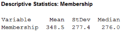
Hence, mean of the number of members per component is 348.5, the median is 276 and the standard deviation is 277.4.
b.
Find the coefficient of skewness.
Identify the shape of the distribution of component size.
b.
Answer to Problem 36CE
The coefficient of skewness is 1.17.
The shape of the distribution of component size is positive skewness.
Explanation of Solution
Calculation:
Step by step procedure to obtain skewness using MINITAB software is given as,
- Choose Stat > Basic Statistics > Graphical Summary.
- In Variables enter the columns Membership.
- Click OK.
Output using MINITAB software is given below:
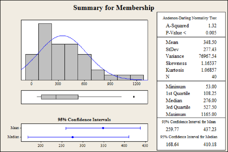
Hence, the value of coefficient of skewness is 1.17.
From the plot, it can be observed that most of the values are extended towards right indicating that distribution of component size is skewed to the right or positively skewed.
c.
Find the first
Find the third quartile.
c.
Answer to Problem 36CE
The first quartile is 108.25.
The third quartile is 527.50.
Explanation of Solution
Calculation:
Location of percentile:
The formula for percentile is,
In the formula, P denotes the location of the percentile and n denotes the total number of observations.
First quartile:
The first quartile represents the 25% of observation lies below first quartile. That is
Substitute,
The position of first quartile is 10.25th value in the dataset.
Hence, the first quartile is 108.25.
Third quartile:
The third quartile represents the 75% of observation lies above third quartile. That is
Substitute,
The position of third quartile is 30.75th value in the dataset.
Hence, the third quartile is 527.50.
d.
Construct a boxplot.
Identify whether there are outliers or not.
Find the components that are outliers.
Find the limits for outliers.
d.
Answer to Problem 36CE
The boxplot is,
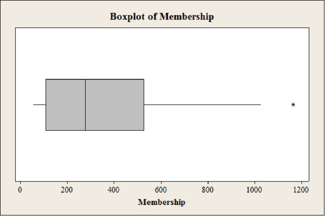
Yes, there are outliers.
The limits for outliers are (0; 1,156.375).
The component that is outlier is California.
Explanation of Solution
Calculation:
Step by step procedure to obtain boxplot using MINITAB software is given as,
- Choose Graph > Boxplot.
- In Graph variables enter the columns Membership.
- Click OK.
In the boxplot, the outlier is represented using asterisk. In the boxplot of data set there is one asterisk representing outliers. Hence, there is one outlier in the dataset.
Limits for detecting outliers:
Any data value beyond the below points are considered as outliers.
Substitute,
Since the membership cannot be negative, the lower point is considered as 0.
The points below 0 and above 1,156.375 are considered as outliers. Hence the limits for outliers are (0; 1,156.375).
The membership corresponding to state ‘California’ is 1,165, which is above the upper limit 1,156.375. This shows that, California is a component of outlier.
Hence, the component that is outlier is California.
Want to see more full solutions like this?
Chapter 4 Solutions
Loose Leaf for Statistical Techniques in Business and Economics


- Review a classmate's Main Post. 1. State if you agree or disagree with the choices made for additional analysis that can be done beyond the frequency table. 2. Choose a measure of central tendency (mean, median, mode) that you would like to compute with the data beyond the frequency table. Complete either a or b below. a. Explain how that analysis can help you understand the data better. b. If you are currently unable to do that analysis, what do you think you could do to make it possible? If you do not think you can do anything, explain why it is not possible.arrow_forward0|0|0|0 - Consider the time series X₁ and Y₁ = (I – B)² (I – B³)Xt. What transformations were performed on Xt to obtain Yt? seasonal difference of order 2 simple difference of order 5 seasonal difference of order 1 seasonal difference of order 5 simple difference of order 2arrow_forwardCalculate the 90% confidence interval for the population mean difference using the data in the attached image. I need to see where I went wrong.arrow_forward
- Microsoft Excel snapshot for random sampling: Also note the formula used for the last column 02 x✓ fx =INDEX(5852:58551, RANK(C2, $C$2:$C$51)) A B 1 No. States 2 1 ALABAMA Rand No. 0.925957526 3 2 ALASKA 0.372999976 4 3 ARIZONA 0.941323044 5 4 ARKANSAS 0.071266381 Random Sample CALIFORNIA NORTH CAROLINA ARKANSAS WASHINGTON G7 Microsoft Excel snapshot for systematic sampling: xfx INDEX(SD52:50551, F7) A B E F G 1 No. States Rand No. Random Sample population 50 2 1 ALABAMA 0.5296685 NEW HAMPSHIRE sample 10 3 2 ALASKA 0.4493186 OKLAHOMA k 5 4 3 ARIZONA 0.707914 KANSAS 5 4 ARKANSAS 0.4831379 NORTH DAKOTA 6 5 CALIFORNIA 0.7277162 INDIANA Random Sample Sample Name 7 6 COLORADO 0.5865002 MISSISSIPPI 8 7:ONNECTICU 0.7640596 ILLINOIS 9 8 DELAWARE 0.5783029 MISSOURI 525 10 15 INDIANA MARYLAND COLORADOarrow_forwardSuppose the Internal Revenue Service reported that the mean tax refund for the year 2022 was $3401. Assume the standard deviation is $82.5 and that the amounts refunded follow a normal probability distribution. Solve the following three parts? (For the answer to question 14, 15, and 16, start with making a bell curve. Identify on the bell curve where is mean, X, and area(s) to be determined. 1.What percent of the refunds are more than $3,500? 2. What percent of the refunds are more than $3500 but less than $3579? 3. What percent of the refunds are more than $3325 but less than $3579?arrow_forwardA normal distribution has a mean of 50 and a standard deviation of 4. Solve the following three parts? 1. Compute the probability of a value between 44.0 and 55.0. (The question requires finding probability value between 44 and 55. Solve it in 3 steps. In the first step, use the above formula and x = 44, calculate probability value. In the second step repeat the first step with the only difference that x=55. In the third step, subtract the answer of the first part from the answer of the second part.) 2. Compute the probability of a value greater than 55.0. Use the same formula, x=55 and subtract the answer from 1. 3. Compute the probability of a value between 52.0 and 55.0. (The question requires finding probability value between 52 and 55. Solve it in 3 steps. In the first step, use the above formula and x = 52, calculate probability value. In the second step repeat the first step with the only difference that x=55. In the third step, subtract the answer of the first part from the…arrow_forward
- If a uniform distribution is defined over the interval from 6 to 10, then answer the followings: What is the mean of this uniform distribution? Show that the probability of any value between 6 and 10 is equal to 1.0 Find the probability of a value more than 7. Find the probability of a value between 7 and 9. The closing price of Schnur Sporting Goods Inc. common stock is uniformly distributed between $20 and $30 per share. What is the probability that the stock price will be: More than $27? Less than or equal to $24? The April rainfall in Flagstaff, Arizona, follows a uniform distribution between 0.5 and 3.00 inches. What is the mean amount of rainfall for the month? What is the probability of less than an inch of rain for the month? What is the probability of exactly 1.00 inch of rain? What is the probability of more than 1.50 inches of rain for the month? The best way to solve this problem is begin by a step by step creating a chart. Clearly mark the range, identifying the…arrow_forwardClient 1 Weight before diet (pounds) Weight after diet (pounds) 128 120 2 131 123 3 140 141 4 178 170 5 121 118 6 136 136 7 118 121 8 136 127arrow_forwardClient 1 Weight before diet (pounds) Weight after diet (pounds) 128 120 2 131 123 3 140 141 4 178 170 5 121 118 6 136 136 7 118 121 8 136 127 a) Determine the mean change in patient weight from before to after the diet (after – before). What is the 95% confidence interval of this mean difference?arrow_forward
- In order to find probability, you can use this formula in Microsoft Excel: The best way to understand and solve these problems is by first drawing a bell curve and marking key points such as x, the mean, and the areas of interest. Once marked on the bell curve, figure out what calculations are needed to find the area of interest. =NORM.DIST(x, Mean, Standard Dev., TRUE). When the question mentions “greater than” you may have to subtract your answer from 1. When the question mentions “between (two values)”, you need to do separate calculation for both values and then subtract their results to get the answer. 1. Compute the probability of a value between 44.0 and 55.0. (The question requires finding probability value between 44 and 55. Solve it in 3 steps. In the first step, use the above formula and x = 44, calculate probability value. In the second step repeat the first step with the only difference that x=55. In the third step, subtract the answer of the first part from the…arrow_forwardIf a uniform distribution is defined over the interval from 6 to 10, then answer the followings: What is the mean of this uniform distribution? Show that the probability of any value between 6 and 10 is equal to 1.0 Find the probability of a value more than 7. Find the probability of a value between 7 and 9. The closing price of Schnur Sporting Goods Inc. common stock is uniformly distributed between $20 and $30 per share. What is the probability that the stock price will be: More than $27? Less than or equal to $24? The April rainfall in Flagstaff, Arizona, follows a uniform distribution between 0.5 and 3.00 inches. What is the mean amount of rainfall for the month? What is the probability of less than an inch of rain for the month? What is the probability of exactly 1.00 inch of rain? What is the probability of more than 1.50 inches of rain for the month? The best way to solve this problem is begin by creating a chart. Clearly mark the range, identifying the lower and upper…arrow_forwardProblem 1: The mean hourly pay of an American Airlines flight attendant is normally distributed with a mean of 40 per hour and a standard deviation of 3.00 per hour. What is the probability that the hourly pay of a randomly selected flight attendant is: Between the mean and $45 per hour? More than $45 per hour? Less than $32 per hour? Problem 2: The mean of a normal probability distribution is 400 pounds. The standard deviation is 10 pounds. What is the area between 415 pounds and the mean of 400 pounds? What is the area between the mean and 395 pounds? What is the probability of randomly selecting a value less than 395 pounds? Problem 3: In New York State, the mean salary for high school teachers in 2022 was 81,410 with a standard deviation of 9,500. Only Alaska’s mean salary was higher. Assume New York’s state salaries follow a normal distribution. What percent of New York State high school teachers earn between 70,000 and 75,000? What percent of New York State high school…arrow_forward
 Big Ideas Math A Bridge To Success Algebra 1: Stu...AlgebraISBN:9781680331141Author:HOUGHTON MIFFLIN HARCOURTPublisher:Houghton Mifflin Harcourt
 Glencoe Algebra 1, Student Edition, 9780079039897...AlgebraISBN:9780079039897Author:CarterPublisher:McGraw Hill
 Holt Mcdougal Larson Pre-algebra: Student Edition...AlgebraISBN:9780547587776Author:HOLT MCDOUGALPublisher:HOLT MCDOUGAL