Chapter 4, Problem 106P

To determine

(a)

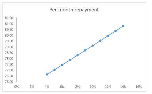
Graphical representation of monthly payment as a function of interest rate.

Answer to Problem 106P

Graphical representation of monthly payment as a function of interest rate.

Explanation of Solution

Given information:

• Loan Amount - $900
• Time period − 1 years
• Rate of Interest − 4-14% per annum

• Capital Recovery Factor:

The capital recovery factor is used to find the uniform annual amount A of a uniform series from a known present worth at the given interest rate i. It is calculated as:

$A=P\left[\frac{i{(1+i)}^n}{{(1+i)}^n-1}\right]=P(A/P,i,n)$.

Calculation:

The loan amount is $900. The monthly payments are to be made, therefore, the rate of interest will be divided by 12, while the time period will be multiplied by 12.

Based on the above information, the following table can be created:

Time Period (in years)	Time Period (in months)	Rate of Interest (compounded annually)	Rate of Interest (compounded monthly)	Loan Amount to be paid	Per month repayment
1	12	4%	0.003	900	76.63
1	12	5%	0.004	900	77.05
1	12	6%	0.005	900	77.46
1	12	7%	0.006	900	77.87
1	12	8%	0.007	900	78.29
1	12	9%	0.008	900	78.71
1	12	10%	0.008	900	79.12
1	12	11%	0.009	900	79.54
1	12	12%	0.010	900	79.96
1	12	13%	0.011	900	80.39
1	12	14%	0.012	900	80.81

Now, the graph will be plotted between the rate of interest compounded annually and per month repayment. The graph will look as:

To determine

(b)

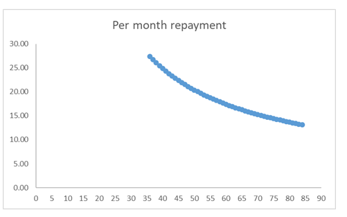
Graphical representation of monthly payment as a function of time period.

Answer to Problem 106P

Graphical representation of monthly payment as a function of interest rate.

Explanation of Solution

Given information:

• Loan Amount - $900
• Rate of Interest − 6% per annum.
• Time period − 36-84 months

• Capital Recovery Factor:

The capital recovery factor is used to find the uniform annual amount A of a uniform series from a known present worth at the given interest rate i. It is calculated as:

$A=P\left[\frac{i{(1+i)}^n}{{(1+i)}^n-1}\right]=P(A/P,i,n)$.

Calculation:

The loan amount is $900. The monthly payments are to be made, therefore, the rate of interest will be divided by 12, while the time period will be multiplied by 12.

Based on this information, following table can be created:

Time Period (in months)	Rate of Interest (compounded annually)	Rate of Interest (compounded monthly)	Loan Amount to be paid	Per month repayment
36	6%	0.005	900	27.38
37	6%	0.005	900	26.70
38	6%	0.005	900	26.06
39	6%	0.005	900	25.46
40	6%	0.005	900	24.88
41	6%	0.005	900	24.33
42	6%	0.005	900	23.81
43	6%	0.005	900	23.31
44	6%	0.005	900	22.84
45	6%	0.005	900	22.38
46	6%	0.005	900	21.95
47	6%	0.005	900	21.53
48	6%	0.005	900	21.14
49	6%	0.005	900	20.75
50	6%	0.005	900	20.39
51	6%	0.005	900	20.04
52	6%	0.005	900	19.70
53	6%	0.005	900	19.37
54	6%	0.005	900	19.06
55	6%	0.005	900	18.76
56	6%	0.005	900	18.47
57	6%	0.005	900	18.19
58	6%	0.005	900	17.91
59	6%	0.005	900	17.65
60	6%	0.005	900	17.40
61	6%	0.005	900	17.15
62	6%	0.005	900	16.92
63	6%	0.005	900	16.69
64	6%	0.005	900	16.47
65	6%	0.005	900	16.25
66	6%	0.005	900	16.04
67	6%	0.005	900	15.84
68	6%	0.005	900	15.65
69	6%	0.005	900	15.45
70	6%	0.005	900	15.27
71	6%	0.005	900	15.09
72	6%	0.005	900	14.92
73	6%	0.005	900	14.75
74	6%	0.005	900	14.58
75	6%	0.005	900	14.42
76	6%	0.005	900	14.26
77	6%	0.005	900	14.11
78	6%	0.005	900	13.96
79	6%	0.005	900	13.82
80	6%	0.005	900	13.68
81	6%	0.005	900	13.54
82	6%	0.005	900	13.41
83	6%	0.005	900	13.28
84	6%	0.005	900	13.15

Now, the graph will be plotted between the time period and per month repayment. The graph will look as: